ChoCG: Poiseuille flow
This example uses ChoCG in Inciter to compute the stationary viscous constant-density (incompressible) laminar flow field in a channel due to an imposed pressure gradient. Since the analytic solution is known the objective is to establish and verify the accuracy of the numerical method and the correctness of the software implementation.
Problem setup
The problem domain consists of a rectangular channel with an imposed streamwise pressure gradient. While the flow field is nominally 2D, we compute it in 3D. The length of the channel in the X coordinate direction is 20 units, its height in Y is , and the width in Z is adjusted to contain a single element in the Z direction depending on the mesh resolution.
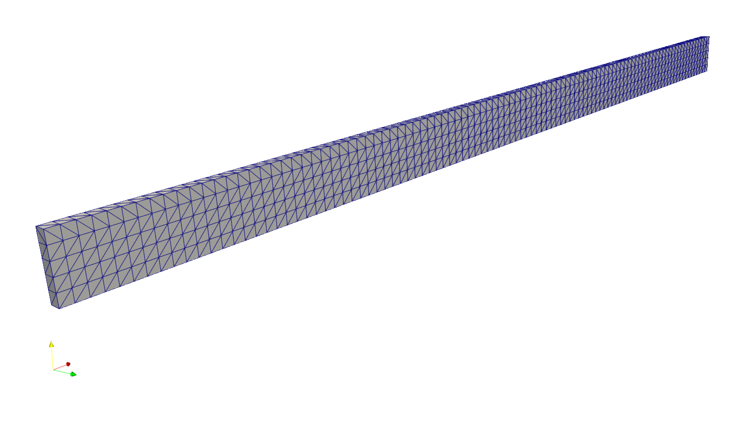
An example mesh is displayed below. The initial and boundary conditions prescribe a pressure gradient of , thus the analytic solution for the streamwise velocity is
where is the pressure and is the dynamic viscosity which yields the laminar Reynolds number as , defined based on the fluid density and the average streamwise velocity . The flow starts with quiescent initial conditions: . At the Z extremes of the computational domain Dirichlet boundary conditions are set to and no-slip/no-penetration boundary conditions, , are applied at the Y extremes representing the channel walls.
 Coarse surface mesh for computing Poiseuille flow, nelem=3K, npoin=1.2K.
Code revision to reproduce
To reproduce the results below, use code revision 9e63b9f and the control file below.
Control file
-- vim: filetype=lua:

print "Poiseuille flow"

-- mesh: poiseuille?tetz.exo
-- plot "diag" u 2:12 w l lw 2 t "L2(err:u)", "" u 2:15 w l lw 2 t "L1(err:u)"

term = 300.0
ttyi = 100

cfl = 0.7

solver = "chocg"
flux = "damp2"
stab = false

part = "rcb"

mat = { dyn_viscosity = 0.01 }

pressure = {
  iter = 500,
  tol = 1.0e-2,
  pc = "jacobi",
  bc_dir = { { 1, 2 },
             { 2, 2 } },
  bc_dirval = { { 1, 2.4 },
                { 2, 0.0 } }
}

problem = {
  name = "poiseuille"
}

bc_noslip = {
  sideset = { 3, 4 }
}

bc_dir = {
  { 5, 0, 1, 1 }
}

fieldout = {
  iter = 1000,
  sideset = { 1, 2, 3 }
}

diag = {
  iter = 10,
  format = "scientific",
  precision = 12
}
Run on a single CPU
Main/inciter -i poiseuille3tetz.exo -c poiseuille_chocg.q -r 10000
Numerical solutions and errors
To estimate the order of convergence, the numerical solution is computed using three different meshes, whose properties of are tabulated below.
| Mesh | Points | Tetrahedra | h |
|---|---|---|---|
| 1 | 1,212 | 3,000 | 0.25 |
| 2 | 4,422 | 12,000 | 0.16 |
| 3 | 16,842 | 48,000 | 0.08 |
Here h is the average edge length.
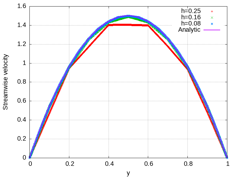
Plotted below are the computed streamwise velocity profiles sampled in the middle of the domain along a line in the Y direction using three different meshes, obtained after the solution has converged to a stationary state.

The L1 and L2 errors are computed as
where is the number of points sampled across the channel, and are the exact and computed solutions at mesh point , and denotes the volume associated to mesh point .
The tables below display the numerical errors for two different types of damping for the advection term. The order of convergence is estimated using the two finer meshes as
where is a mesh index.
Errors (sampled along the centerline in the cross-stream direction) and convergence rates using second-order damping for advection and forward Euler time stepping.
| Mesh | h | L1(err) | L2(err) |
|---|---|---|---|
| 1 | 0.25 | 0.0416288 | 0.0451145 |
| 2 | 0.16 | 0.0090595 | 0.0101426 |
| 3 | 0.08 | 0.0019338 | 0.0021336 |
| p | 2.228 | 2.2491 |