ChoCG: Slotted cylinder
This example uses ChoCG in Inciter to compute a solid-body rotation problem. Such tests are frequently used to evaluate and compare numerical schemes for convection-dominated problems.
Here we evaluate the numerical method using Zalesak's slotted cylinder problem [1], augmented by Leveque [2] in order to examine the resolution of both smooth and discontinuous profiles.
Equations solved
In this example we numerically solve the linear advection equation of a passive scalar, denoted by , (e.g., a normalized concentration of a pollutant), coupled to the Navier-Stokes equations governing viscous Newtonian constant-density flow, see also ChoCG, as
where is the velocity vector, is the pressure, and both the pressure and the viscosity have been normalized by the (constant) density. Furthermore, , is a source term that arise from the application of the method of manufactured solutions, used for verification only. This source term is zero when computing practical engineering problems.
Problem setup
The initial configuration for the scalar field, , is depicted in the figure below.
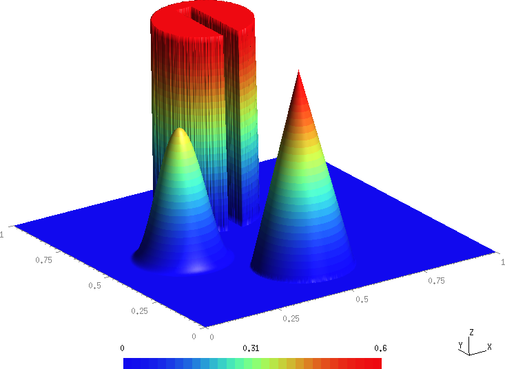
While this is a 2D test problem, we calculate it on a 3D domain with the extents . Since we are only interested in the evolution of the scalar, we prescribe the source term that yields a stationary flow with a prescribed rotational velocity field as
Each solid body lies within a radius centered at a point . In the rest of the domain the solution is initially zero. The shapes of the three bodies can be expressed in terms of the normalized distance function for the respective reference point
The center of the slotted cylinder is located at and its geometry is given by
The corresponding analytical expression for the conical body is
while the shape and location of the hump reads
The initial conditions are sampled from the analytic solutions above. We set inhomogeneous Dirichlet boundary conditions for all variables on the sides of the domain with normals in the or directions, sampling their analytic solutions. On the sides with normals in the direction, the flow variables are sampled from their analytic solutions, while for the scalar, homogeneous Neumann conditions are enforced.
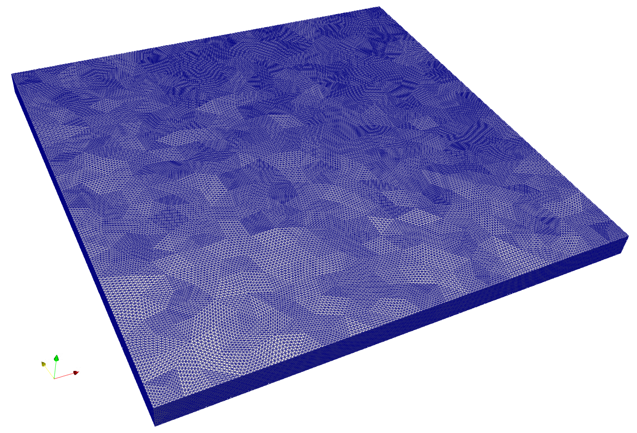 Surface mesh for computing the slotted cylinder test problem, nelem=1.9M, npoin=349K.
Code revision to reproduce
To reproduce the results below, use code revision becc101 and the control file below.
Control file
-- vim: filetype=lua:

print "Scalar transport: slotted cylinder, cone, hump"

term = math.pi
ttyi = 10
cfl = 0.1

solver = "chocg"
flux = "damp4"
rk = 4

part = "rcb"

problem = {
  name = "slot_cyl"
}

pressure = {
  iter = 1000,
  tol = 1.0e-2,
  pc = "jacobi",
  hydrostat = 0
}

bc_dir = {
  { 1, 1, 1, 1, 1 },
  { 2, 1, 1, 1, 1 },
  { 3, 1, 1, 1, 1 },
  { 4, 1, 1, 1, 0 },
  { 5, 1, 1, 1, 1 },
  { 6, 1, 1, 1, 0 }
}

fieldout = {
  iter = 500
}

diag = {
  iter = 1,
  format = "scientific",
  precision = 12
}
Run using on 32 CPUs
./charmrun +p32 Main/inciter -i unitsquare_01_1.9M.exo -c slot_cyl.q
Visualization
ParaView can be used for interactive visualization of the numerically computed fields as
paraview out.e-s.0.32.0Results
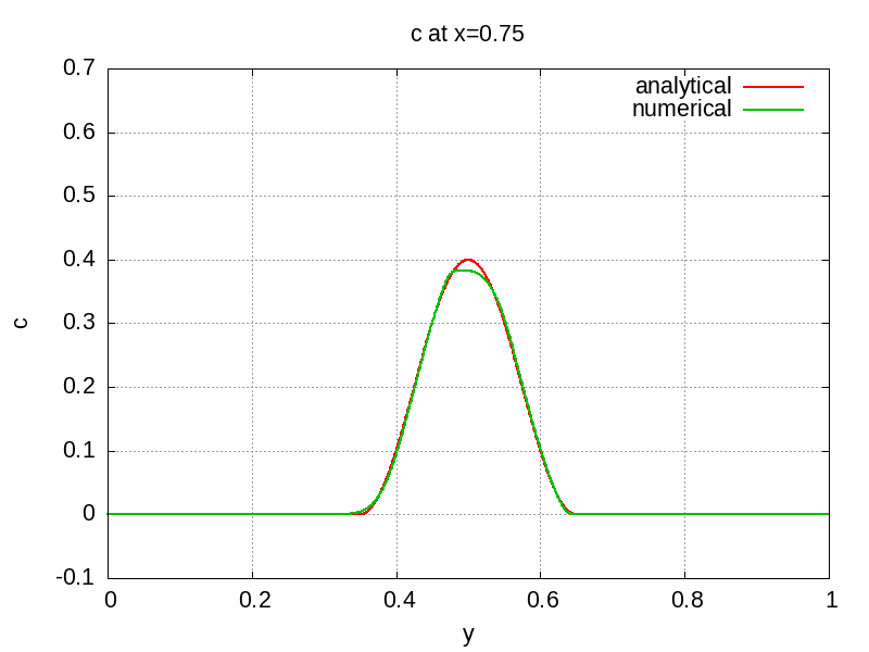
The scalar field after half revolution is depicted below with several line-outs at various locations so the solution can be compared to the analytic solution.


References
- S.T. Zalesak, Fully multidimensional flux-corrected transport algorithms for fluids, J. Comput. Phys. 31,3, p.335-362, 1979.
- R.J. Leveque, High-resolution conservative algorithms for advection in incompressible flow, SIAM J. on Numerical Analysis, 33, p.627-665 1996.