How to use Charm++'s Projections

How to analyze Xyst performance with Charm++'s Projections tool

To enable performance analysis of Xyst with Charm++ do

git clone https://codeberg.org/xyst/xyst.git && cd xyst
mkdir build && cd build
cmake -DCMAKE_C_COMPILER=mpicc -DCMAKE_CXX_COMPILER=mpicxx -GNinja -DCHARM_OPTS="-DTRACING=true -DTRACING_COMMTHREAD=true" -Wno-dev -DRUNNER_ARGS="--bind-to none -oversubscribe" -DPOSTFIX_RUNNER_ARGS=+setcpuaffinity -DEXTRA_LINK_ARGS="-tracemode projections" ../src
ninja

The above will build Charm++ enabling performance tracing and will pass an extra link argument to Xyst executables. This instructs Charm++ to produce information about all Charm++ events, e.g., entry method calls and message packing, during the execution of Xyst executables.

Once the above went fine, performance can be analyzed by first collecting some data:

./charmrun +p32 Main/inciter -i ../../tmp/problems/sedov/sedov01.exo -c ../../tmp/problems/sedov/sedov_riecg.q

Running as 32 OS processes:  Main/inciter -i ../../tmp/problems/sedov/sedov01.exo -c ../../tmp/problems/sedov/sedov_riecg.q
charmrun>  /usr/bin/setarch x86_64 -R  mpirun -np 32  Main/inciter -i ../../tmp/problems/sedov/sedov01.exo -c ../../tmp/problems/sedov/sedov_riecg.q
Charm++> Running on MPI version: 3.1      
Charm++> level of thread support used: MPI_THREAD_SINGLE (desired: MPI_THREAD_SINGLE)
Charm++> Running in non-SMP mode: 32 processes (PEs)
Converse/Charm++ Commit ID: fa84486       
Charm++: Tracemode Projections enabled.   
Trace: traceroot: Main/inciter            
Isomalloc> Synchronized global address space.
CharmLB> Load balancer assumes all CPUs are same.
Xyst> Load balancing off                  
Charm++> Running on 1 hosts (2 sockets x 16 cores x 1 PUs = 32-way SMP)
Charm++> cpu topology info is gathered in 0.002 seconds.
...

This run will produce log and sts files in the build folder where the executable resides. Projections can then be used to analyze performance data in detail. Example screenshots are displayed below.

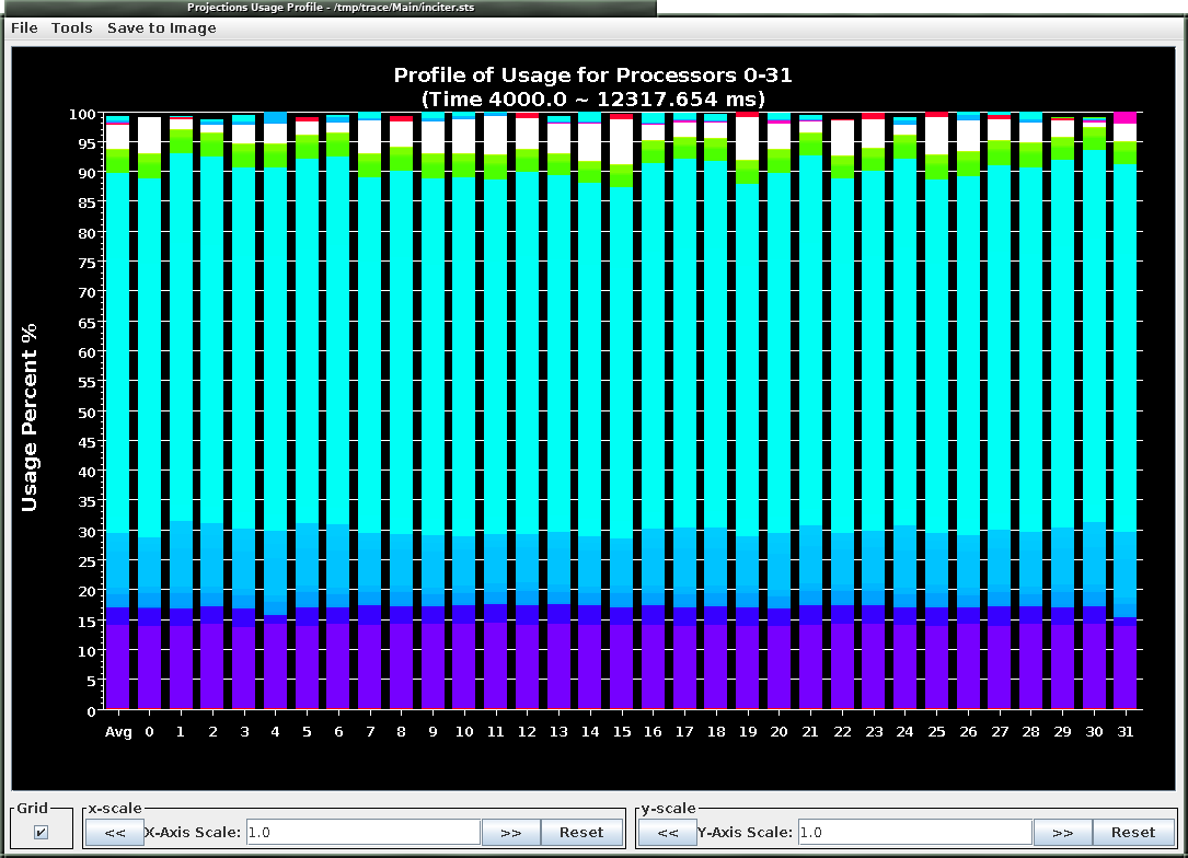Example average CPU utilization profile between 4s and 12.3s of a run taking 50 time steps with the RieCG solver computing the Sedov problem on 32 CPUs. The colors correspond to various tasks during a time step.

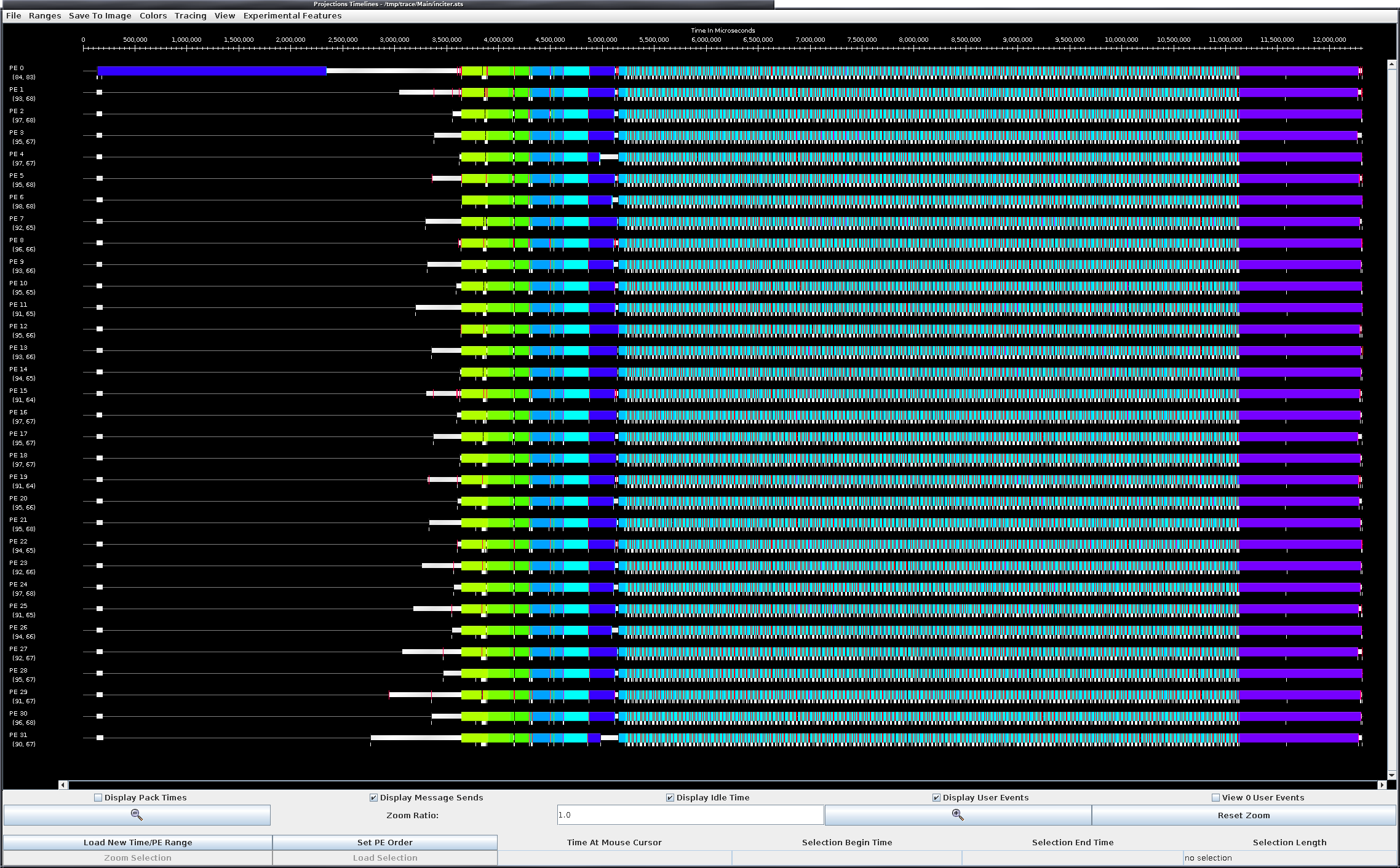Example projection timelines during the same simulation as above. The vertical axis displays the 32 CPUs and the horizontal axis measures wall-clock time. The colors correspond to various tasks. Clearly visible is the time stepping in the middle of the figure in mostly white and light blue, followed by saving the checkpoint at the end of time stepping in purple.