KozCG: Rayleigh-Taylor unstable configuration
This example uses KozCG in Inciter to compute a problem whose analytic solution is known, therefore it can be used to verify the accuracy of the numerical method and the correctness of the software implementation.
The purpose of this test case is to assess time dependent fluid motion in the presence of Rayleigh-Taylor unstable conditions, i.e., opposing density and pressure gradients. The derivation of this test problem is given in [1].
Equations solved
The system of equation solved is
detailed at the KozCG page describing its numerical method, with the exact solution
and the source terms
For more details, see Papers.
Problem setup
The simulation domain is a cube centered around the point {0,0,0}. The initial conditions are sampled from the analytic solution at t=0. We set Dirichlet boundary conditions on the sides of the cube, sampling the analytic solution. The numerical solution is time-dependent. The simulation was run for a single time unit computing the numerical errors during time stepping and the errors at t=1 are used to assess the convergence rate. A time step of 0.001 was used for the coarsest mesh and was successively halved for the finer meshes.
To estimate the order of convergence, the numerical solution is computed using three different meshes, whose properties of are tabulated below, where h is the average edge length.
| Mesh | Points | Tetrahedra | h |
|---|---|---|---|
| 750K | 132,651 | 750,000 | 0.02 |
| 6M | 1,030,301 | 6,000,000 | 0.01 |
| 48M | 8,120,601 | 48,000,000 | 0.005 |
Code revision to reproduce
To reproduce the results below, use code revision 8c9d1db and the control file below.
Control file
-- vim: filetype=lua:

print "Euler equations computing non-stationary Rayleigh-Taylor"

term = 3.0
ttyi = 10

solver = "kozcg"
fct = false

dt = 0.001      -- 750K
--dt = 0.0005     --   6M
--dt = 0.00025      --  48M

part = "rcb"

problem = {
  name = "rayleigh_taylor",
  alpha = 1.0,
  beta = { 1.0, 1.0, 1.0 },
  p0 = 1.0,
  r0 = 1.0,
  kappa = 1.0,
}

mat = { spec_heat_ratio = 5/3 }

bc_dir = {
  { 1, 1, 1, 1, 1, 1 },
  { 2, 1, 1, 1, 1, 1 },
  { 3, 1, 1, 1, 1, 1 },
  { 4, 1, 1, 1, 1, 1 },
  { 5, 1, 1, 1, 1, 1 },
  { 6, 1, 1, 1, 1, 1 }
}

fieldout = {
  iter = 1000
}

diag = {
  iter = 1,
  format = "scientific"
}
Run using the 750K mesh on 32 CPUs
./charmrun +p32 Main/inciter -i unitcube_750K.exo -c rayleigh_taylor.q
Visualization
ParaView can be used for interactive visualization of the numerically computed fields as
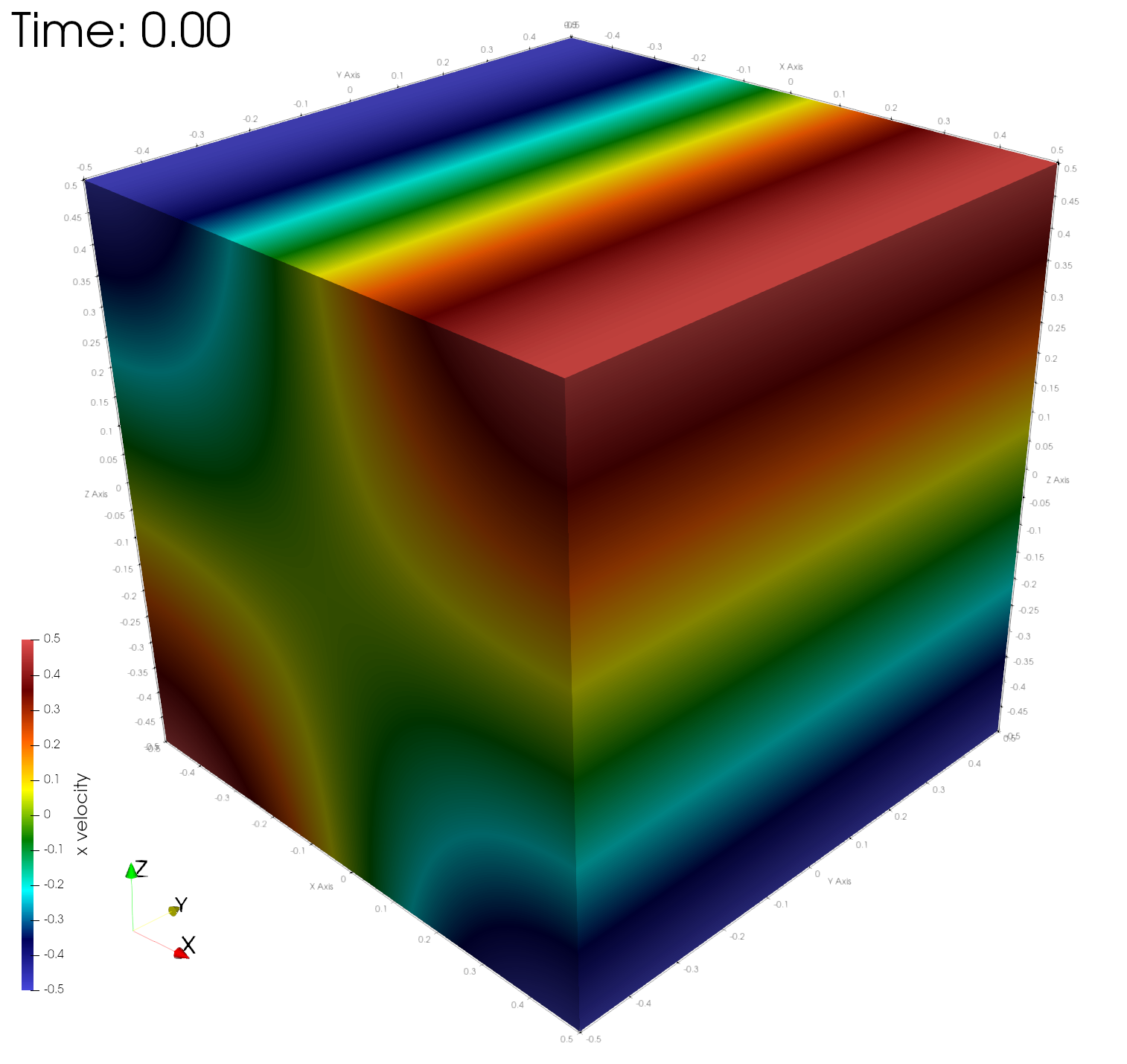
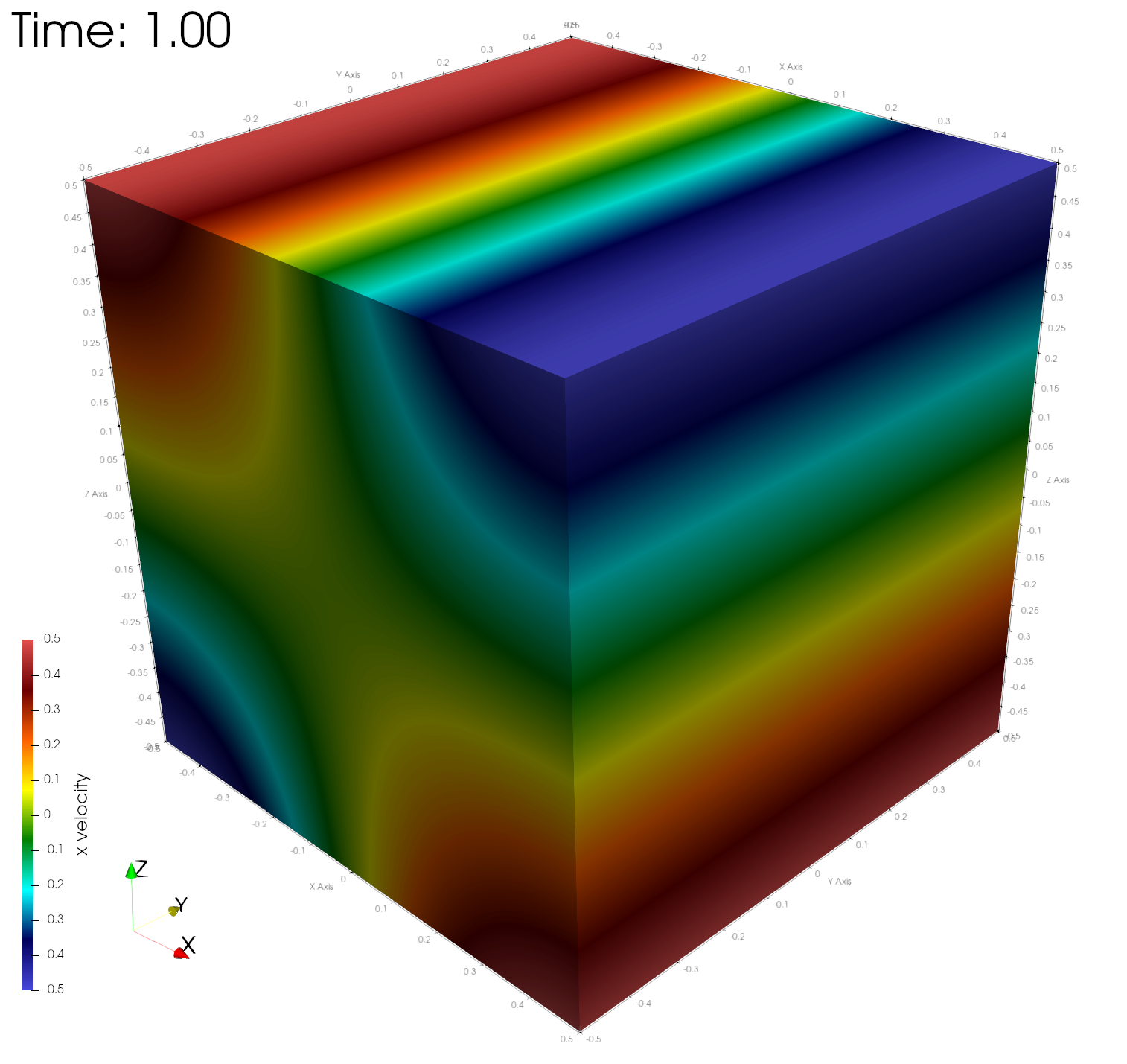
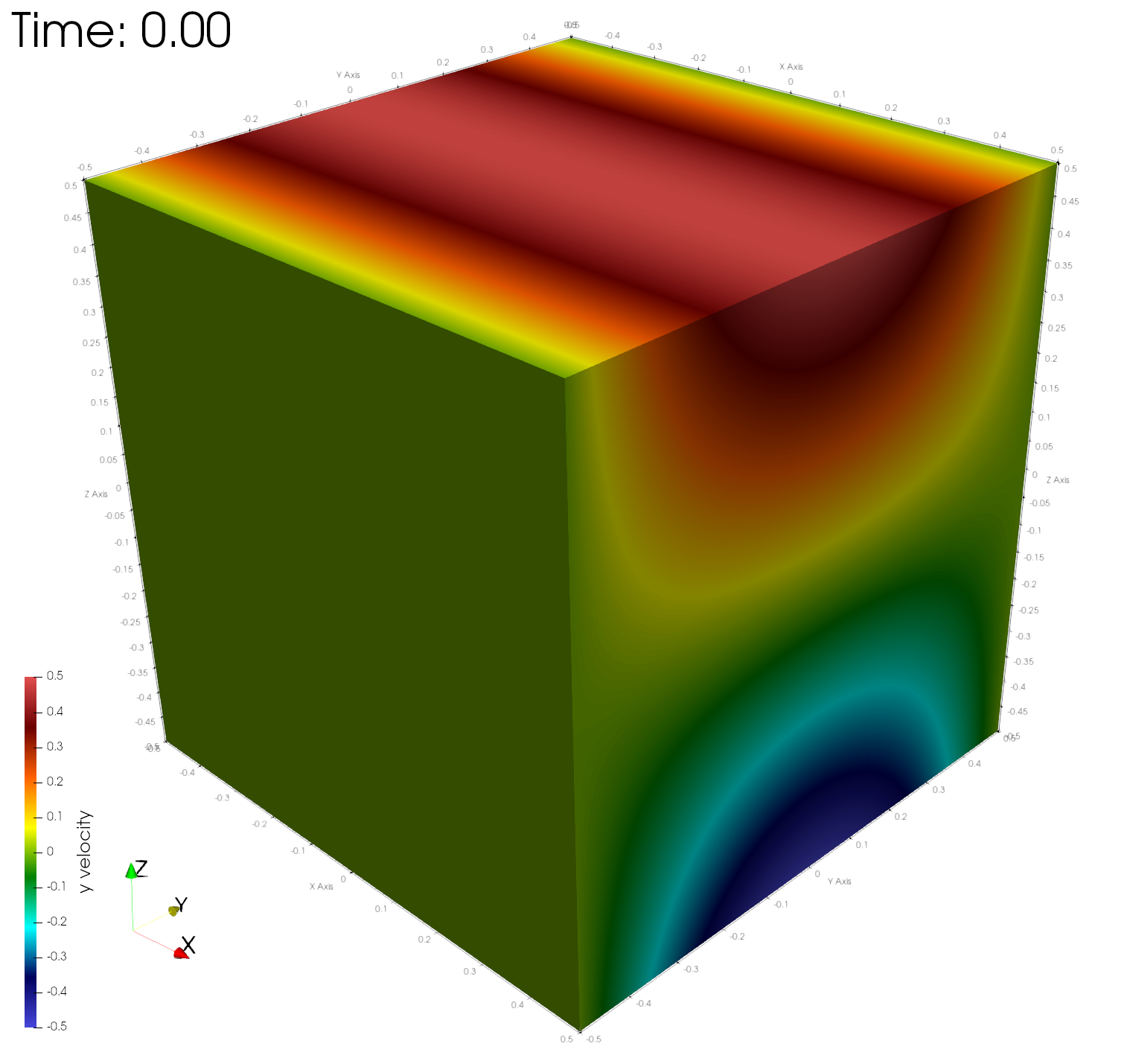
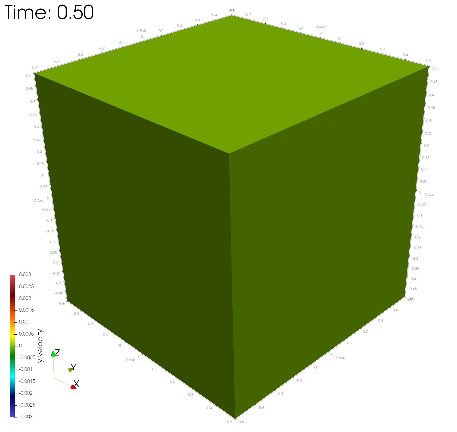
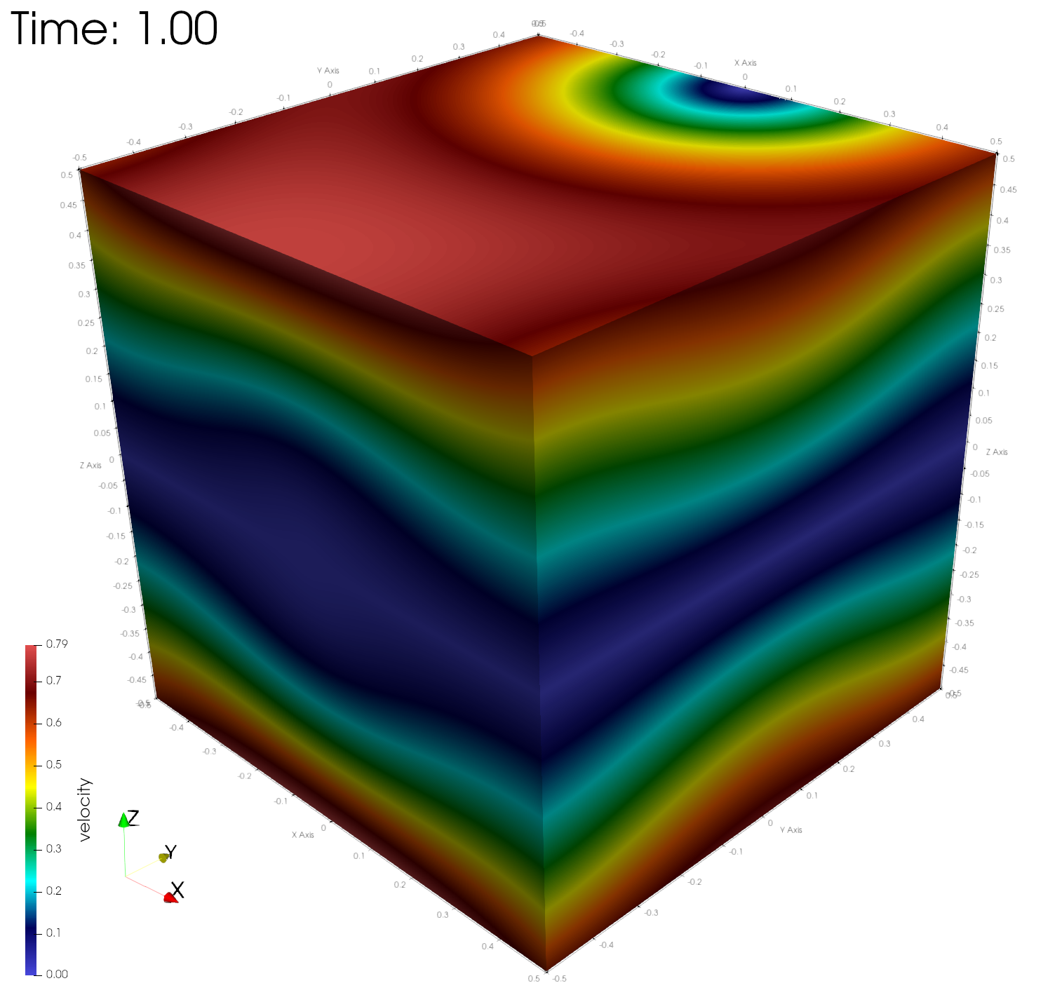
paraview out.e-s.0.32.0The figures below depict the velocity field at the surface at different simulation times, showing the reversal of the velocity components in time, indicating the spatial and temporal dynamics of the velocity field.

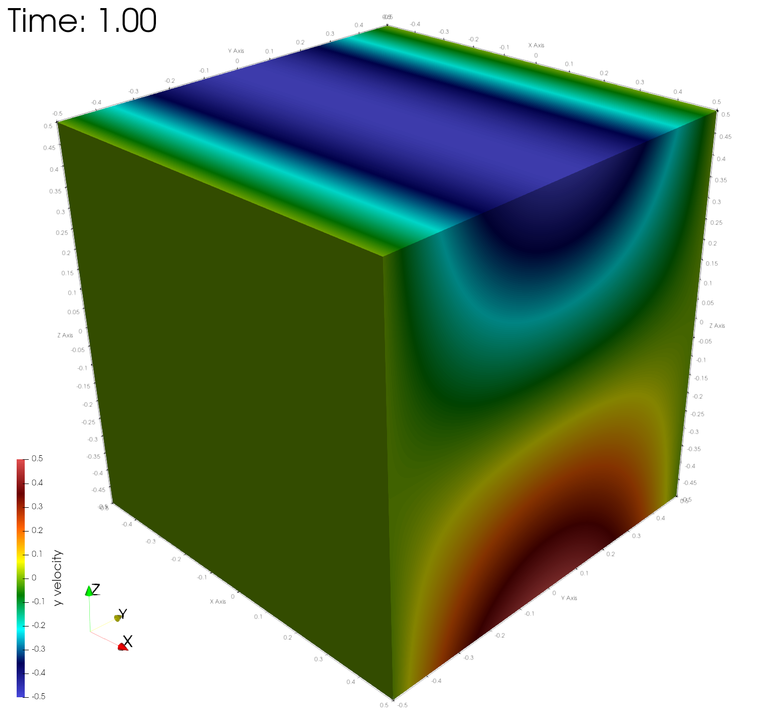
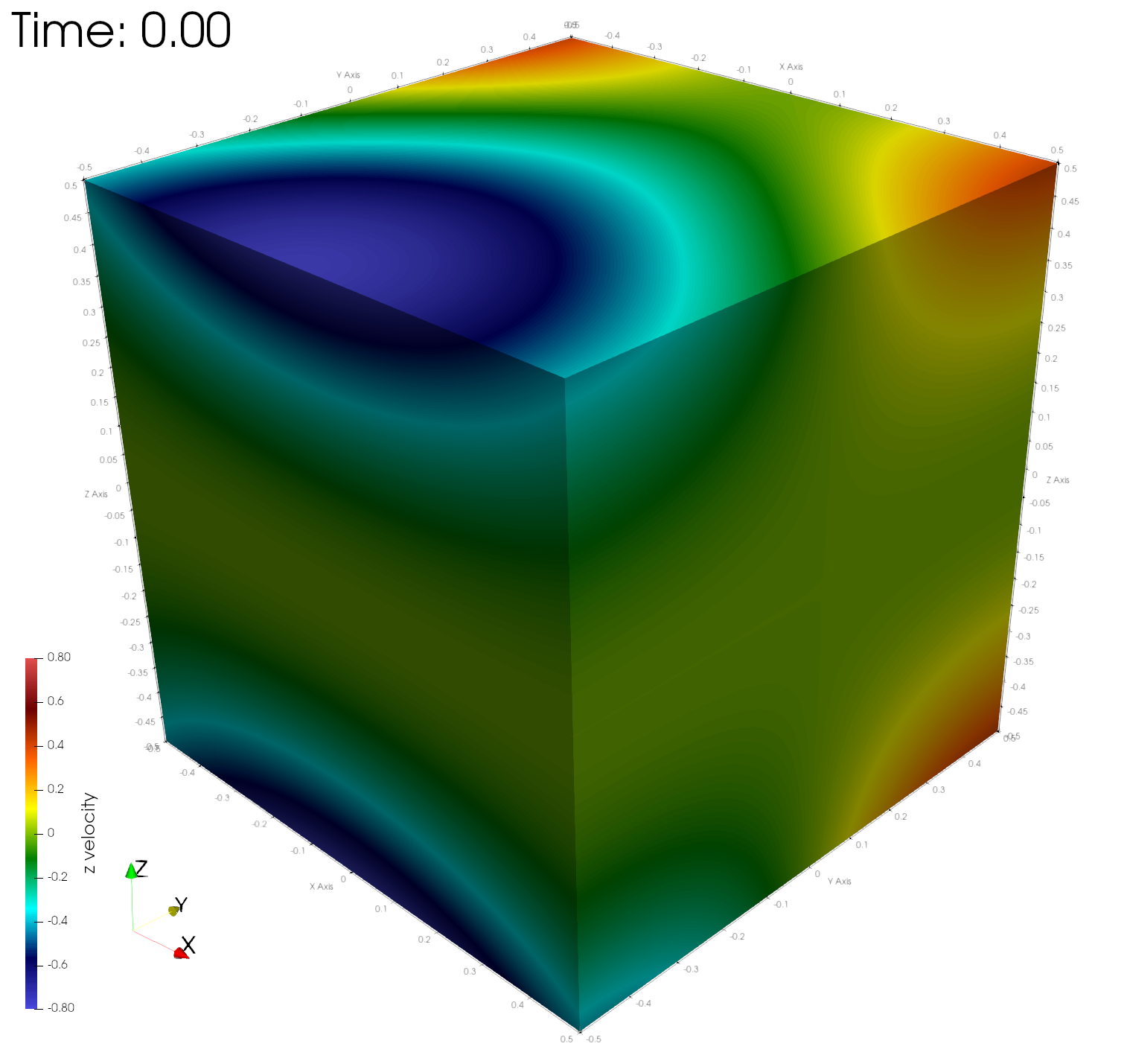
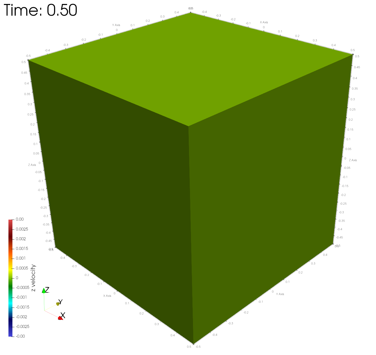
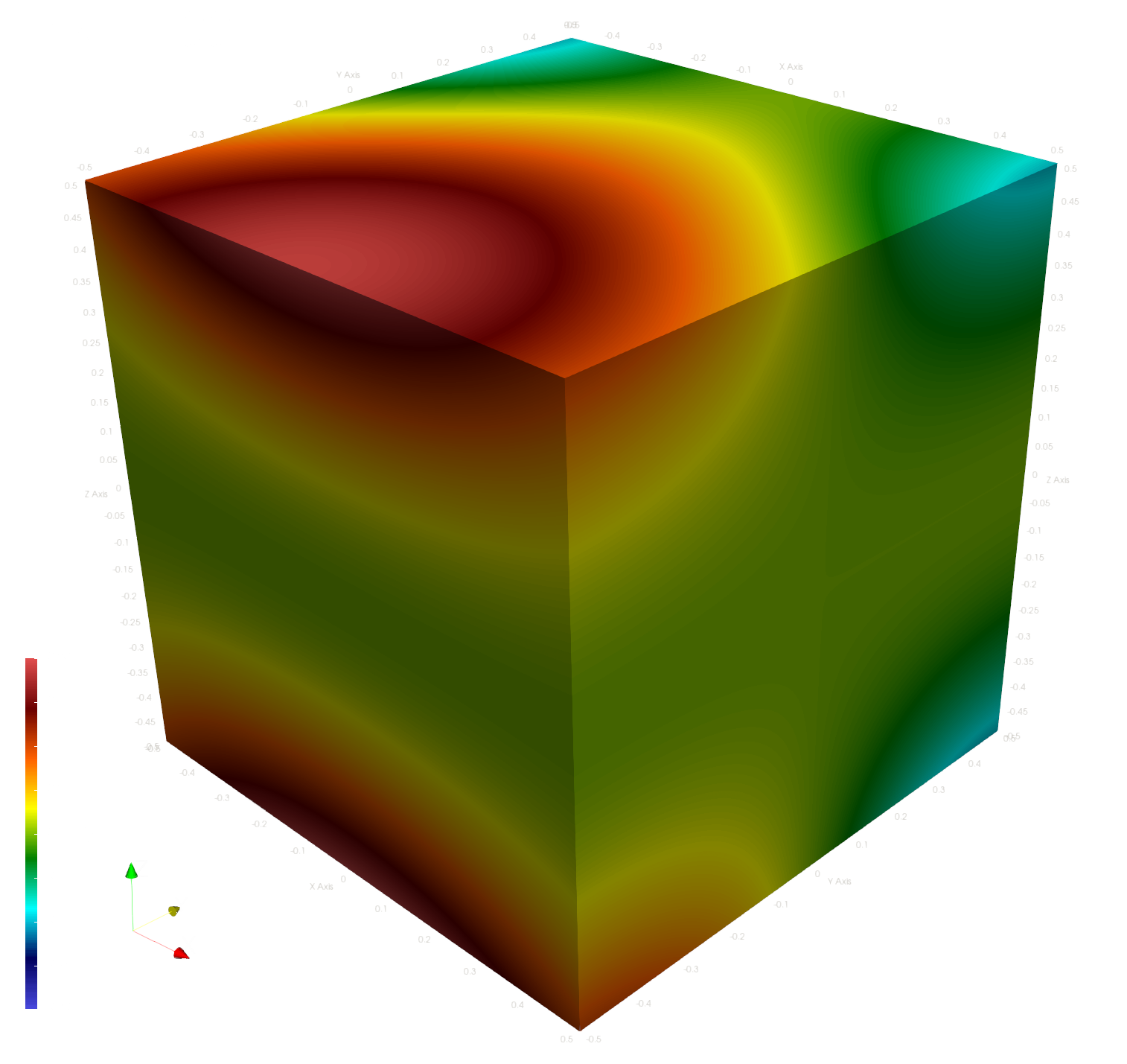
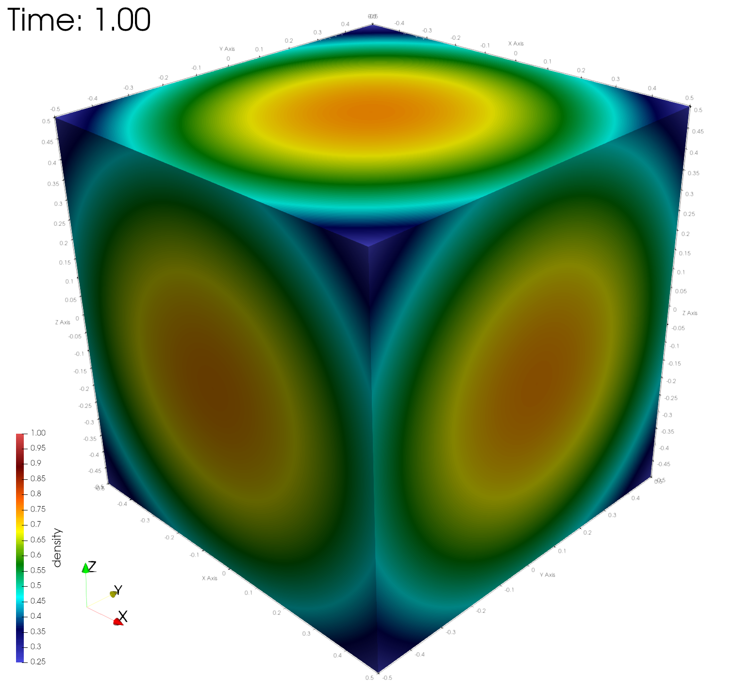
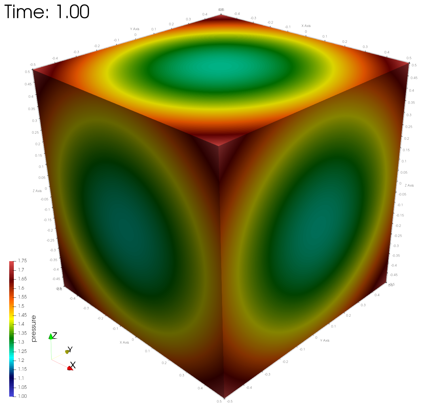
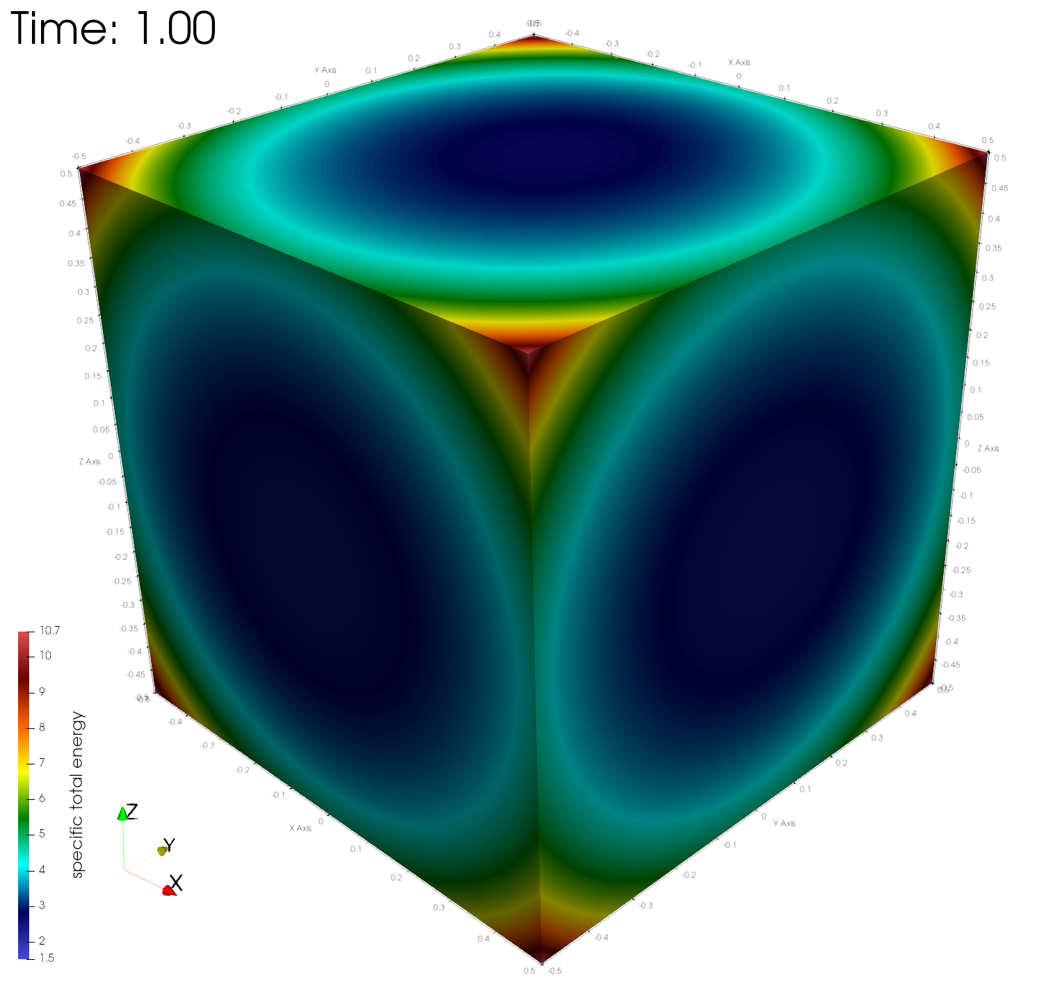
The figures below show the density, pressure, energy, and velocity on the surface at the final simulation time.
Numerical errors and convergence rate
The table below shows the numerical L1 errors of the flow quantities computed. The L1 error is computed as
where n is the total number of points of the mesh, and are the exact and computed solutions at mesh point v, and denotes the volume associated to mesh point v. The order of convergence is estimated as
where m is a mesh index. The following table summarizes the L1 errors in all flow variables at t=1.
| Mesh | L1(r) | L1(u) | L1(v) | L1(w) | L1(e) |
|---|---|---|---|---|---|
| 750K | 1.09e-3 | 6.65e-4 | 9.17e-4 | 7.21e-4 | 5.22e-3 |
| 6M | 3.08e-4 | 1.85e-4 | 2.50e-4 | 1.98e-4 | 1.54e-3 |
| 48M | 8.03e-5 | 4.93e-5 | 6.38e-5 | 5.13e-5 | 4.13e-4 |
| p | 1.94 | 1.91 | 1.97 | 1.95 | 1.90 |
Here r, u, v, w, and e are the fluid density, velocity in the x, y, z directions, and the internal energy, respectively. The order of convergence approaches the expected value of 2.0.
References
- J. Waltz and T.R. Canfield and N.R. Morgan and L.D. Risinger and J.G. Wohlbier, Manufactured solutions for the three-dimensional Euler equations with relevance to Inertial Confinement Fusion, Journal of Computational Physics, 267, 196–209, 2014.