KozCG: Taylor-Green vortex
This example uses KozCG in Inciter to compute a problem whose analytic solution is known, therefore it can be used to verify the accuracy of the numerical method and the correctness of the software implementation.
We compute 3D simulations of the 2D Taylor-Green vortex, see e.g., [1]. This is a time-invariant solution of the problem. A similar configuration was also computed in [2,3] on a different, practically 2D, domain.
Equations solved
The system of equation solved is
detailed at the KozCG page describing its numerical method, with the exact solution
and the source terms
For more details, see Papers.
Problem setup
The simulation domain is a cube centered around the point {0,0,0}. The initial conditions are sampled from the analytic solution at t=0. We set Dirichlet boundary conditions on the sides of the cube, sampling the analytic solution. The numerical solution does not depend on time and approaches steady state due to the source term which ensures equilibrium in time. As the numerical solution approaches a stationary state, the numerical errors in the flow variables converge to stationary values, determined by the combination of spatial and temporal errors which are measured and assessed. The simulation was run for a single time unit computing the numerical errors. A time step of 0.002 was used for the coarsest mesh and was successively halved for the finer meshes.
To estimate the order of convergence, the numerical solution is computed using three different meshes, whose properties of are tabulated below.
| Mesh | Points | Tetrahedra | h |
|---|---|---|---|
| 750K | 132,651 | 750,000 | 0.02 |
| 6M | 1,030,301 | 6,000,000 | 0.01 |
| 48M | 8,120,601 | 48,000,000 | 0.005 |
Here h is the average edge length.
Code revision to reproduce
To reproduce the results below, use code revision 8c9d1db and the control file below.
Control file
-- vim: filetype=lua:

print "Euler equations computing stationary Taylor-Green"

term = 2.0
ttyi = 10

solver = "kozcg"
fct = false

dt = 0.002      -- 750K
--dt = 0.001      --   6M
--dt = 0.0005      --  48M

part = "rcb"

problem = {
  name = "taylor_green"
}

mat = { spec_heat_ratio = 5/3 }

bc_dir = {
  { 1, 1, 1, 1, 1, 1 },
  { 2, 1, 1, 1, 1, 1 },
  { 3, 1, 1, 1, 1, 1 },
  { 4, 1, 1, 1, 1, 1 },
  { 5, 1, 1, 1, 1, 1 },
  { 6, 1, 1, 1, 1, 1 }
}

fieldout = {
  iter = 1000
}

diag = {
  iter = 1,
  format = "scientific"
}
Run using the 750K mesh on 32 CPUs
./charmrun +p32 Main/inciter -i unitcube_750K.exo -c taylor_green.q
Visualization
ParaView can be used for interactive visualization of the numerically computed fields as
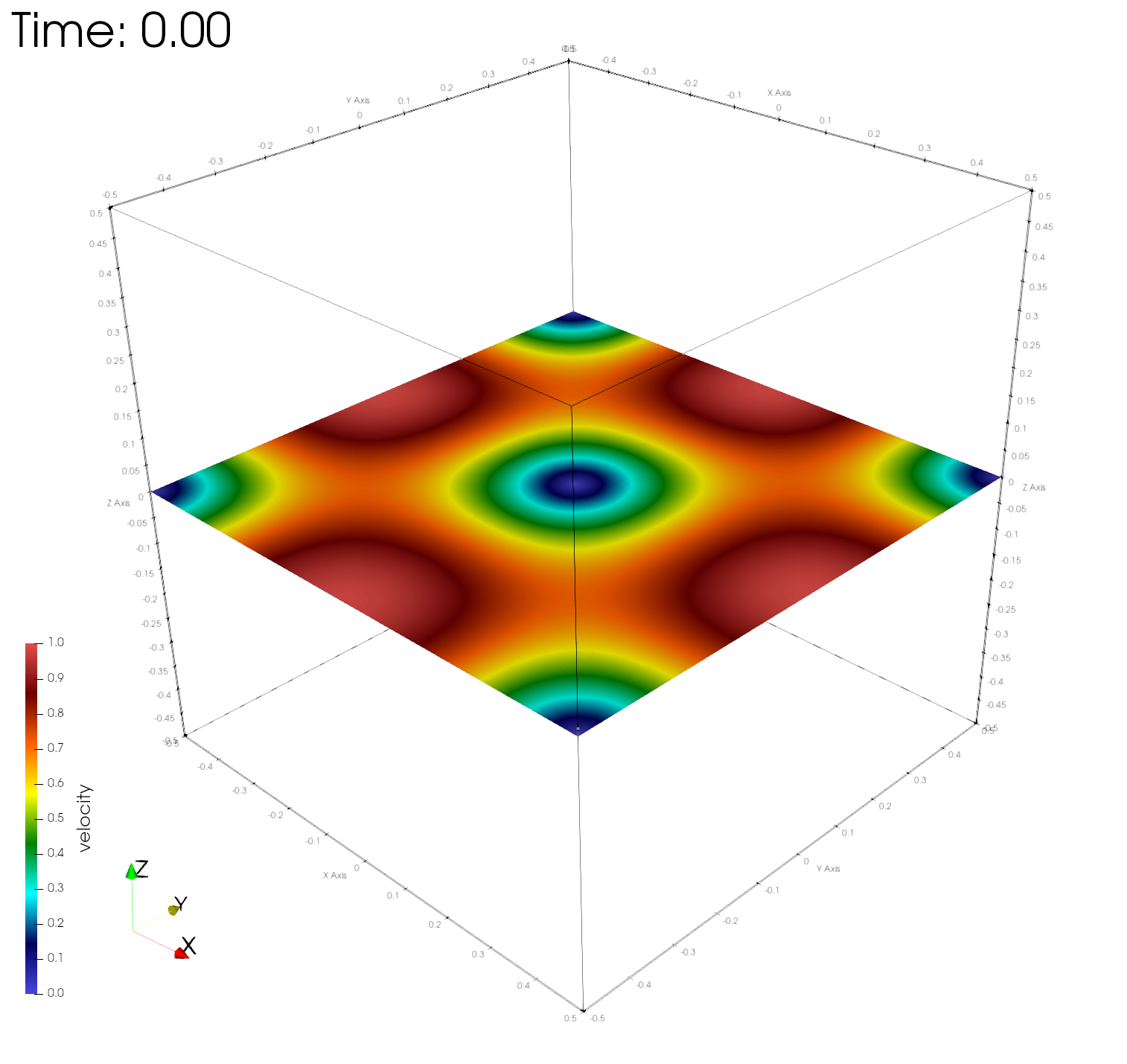
paraview out.e-s.0.32.0The figures below show the velocity magnitudes across a center plane at different simulation times, demonstrating time-invariance of the numerical solution.


Numerical errors and convergence rate
The table below shows the numerical L1 errors of the flow quantities computed. The L1 error is computed as
where n is the number of points, and are the exact and computed solutions at mesh point v, and denotes the volume associated to mesh point v. The order of convergence is estimated as
where m is a mesh index. The following table summarizes the L1 errors in all flow variables at the stationary state.
| Mesh | L1(r) | L1(u) | L1(v) | L1(w) | L1(e) |
|---|---|---|---|---|---|
| 750K | 1.28e-5 | 5.19e-5 | 3.31e-4 | 2.39e-5 | 1.92e-4 |
| 6M | 2.41e-6 | 7.28e-6 | 5.00e-5 | 3.40e-6 | 4.04e-5 |
| 48M | 5.41e-7 | 1.38e-6 | 8.33e-6 | 7.10e-7 | 1.02e-5 |
| p | 2.16 | 2.40 | 2.59 | 2.26 | 1.99 |
Here r, u, v, w, and e are the fluid density, velocity in the x, y, z directions, and the internal energy, respectively. As expected, the asymptotic convergence of the computed numerical solution in all variables approaches 2.
References
- J.R. Kamm, Enhanced verification test suite for phyics simulation codes, LA-14379, SAND2008-7813, 2008.
- J. Waltz, Microfluidics simulation using adaptive unstructured grids, International Journal for Numerical Methods in Fluids, 46, 9, 939-960, 2004.
- J. Waltz, T.R. Canfield, N.R. Morgan, L.D. Risinger, J.G. Wohlbier, Verification of a three-dimensional unstructured finite element method using analytic and manufactured solutions, Computers & Fluids, 81: 57-67, 2013.