KozCG: Vortical flow
This example uses KozCG in Inciter to compute a problem whose analytic solution is known, therefore it can be used to verify the accuracy of the numerical method and the correctness of the software implementation.
The purpose of this problem is to test velocity errors generated by spatial operators in the presence of 3D vorticity and in particular the superposition of planar and vortical flows, analogous to vorticity stretching. The derivation of this test problem, using the method of manufactured solutions, is given in [1], preceded by a simplified version published in [2]. The combination of vorticity and velocity gradients is a fundamental source of kinetic energy in flows that transition to shear-driven turbulence, and hence an important ingredient of computing many practical engineering and atmospheric flows.
Equations solved
The system of equation solved is
detailed at the KozCG page describing its numerical method, with the exact solution
and the source terms
For more details, see Papers.
Problem setup
The simulation domain is a cube centered around the point {0,0,0}. The initial conditions are sampled from the analytic solution at t=0. We set Dirichlet boundary conditions on the sides of the cube, sampling the analytic solution. The numerical solution does not depend on time and approaches steady state due to the source term which ensures equilibrium in time. As the numerical solution approaches a stationary state, the numerical errors in the flow variables converge to stationary values, determined by the combination of spatial and temporal errors which are measured and assessed.
Code revision to reproduce
To reproduce the results below, use code revision 8c9d1db and the control file below.
Control file
-- vim: filetype=lua:

print "Euler equations computing vortical flow"

term = 3.0
ttyi = 10

solver = "kozcg"
fct = false

dt = 0.002      -- 750K
--dt = 0.001      --   6M
--dt = 0.0005      --  48M

part = "rcb"

problem = {
  name = "vortical_flow",
  alpha = 1.0,
  kappa = 1.0,
  p0 = 10.0,
}

mat = { spec_heat_ratio = 5/3 }

bc_dir = {
  { 1, 1, 1, 1, 1, 1 },
  { 2, 1, 1, 1, 1, 1 },
  { 3, 1, 1, 1, 1, 1 },
  { 4, 1, 1, 1, 1, 1 },
  { 5, 1, 1, 1, 1, 1 },
  { 6, 1, 1, 1, 1, 1 }
}

fieldout = {
  iter = 1000
}

diag = {
  iter = 1,
  format = "scientific"
}
Run using the 750K mesh on 32 CPUs
./charmrun +p32 Main/inciter -i unitcube_750K.exo -c vortical_flow.q
Visualization
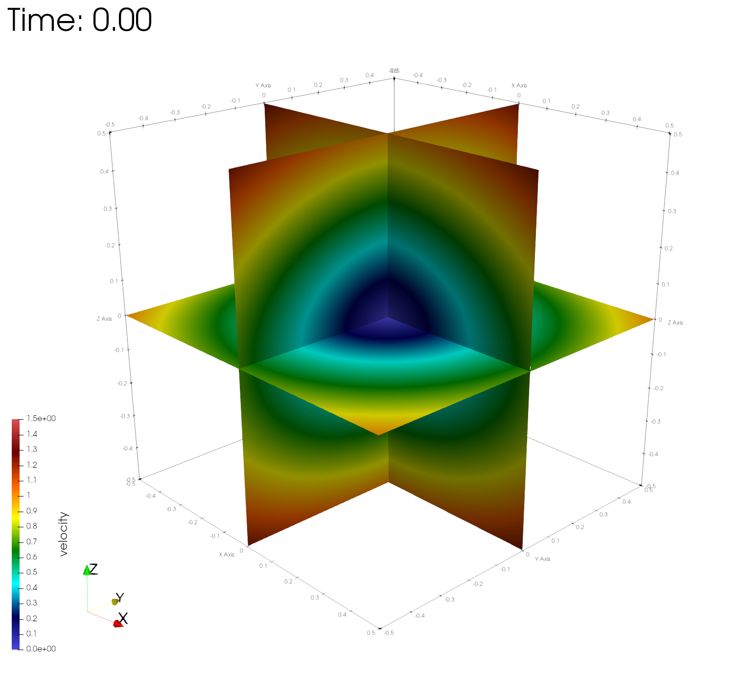
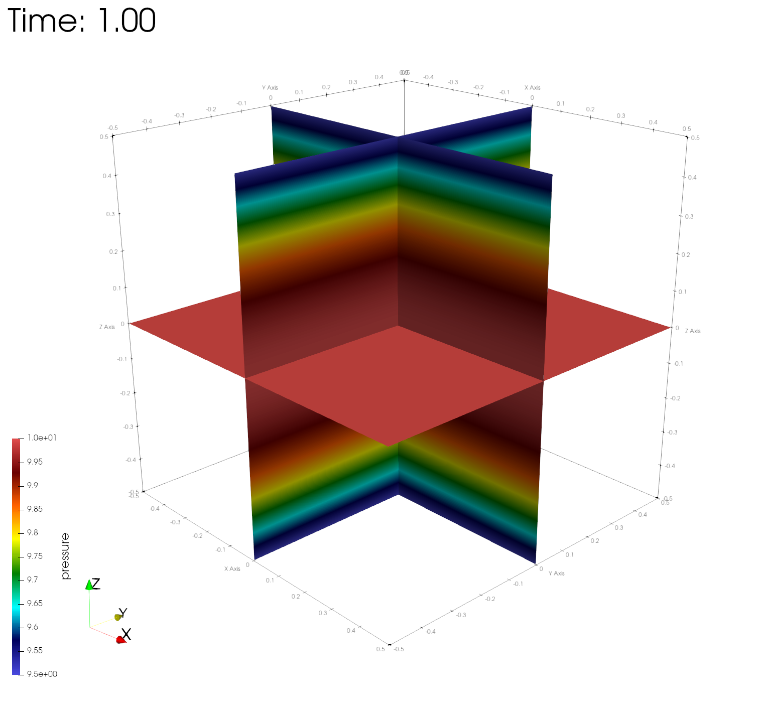
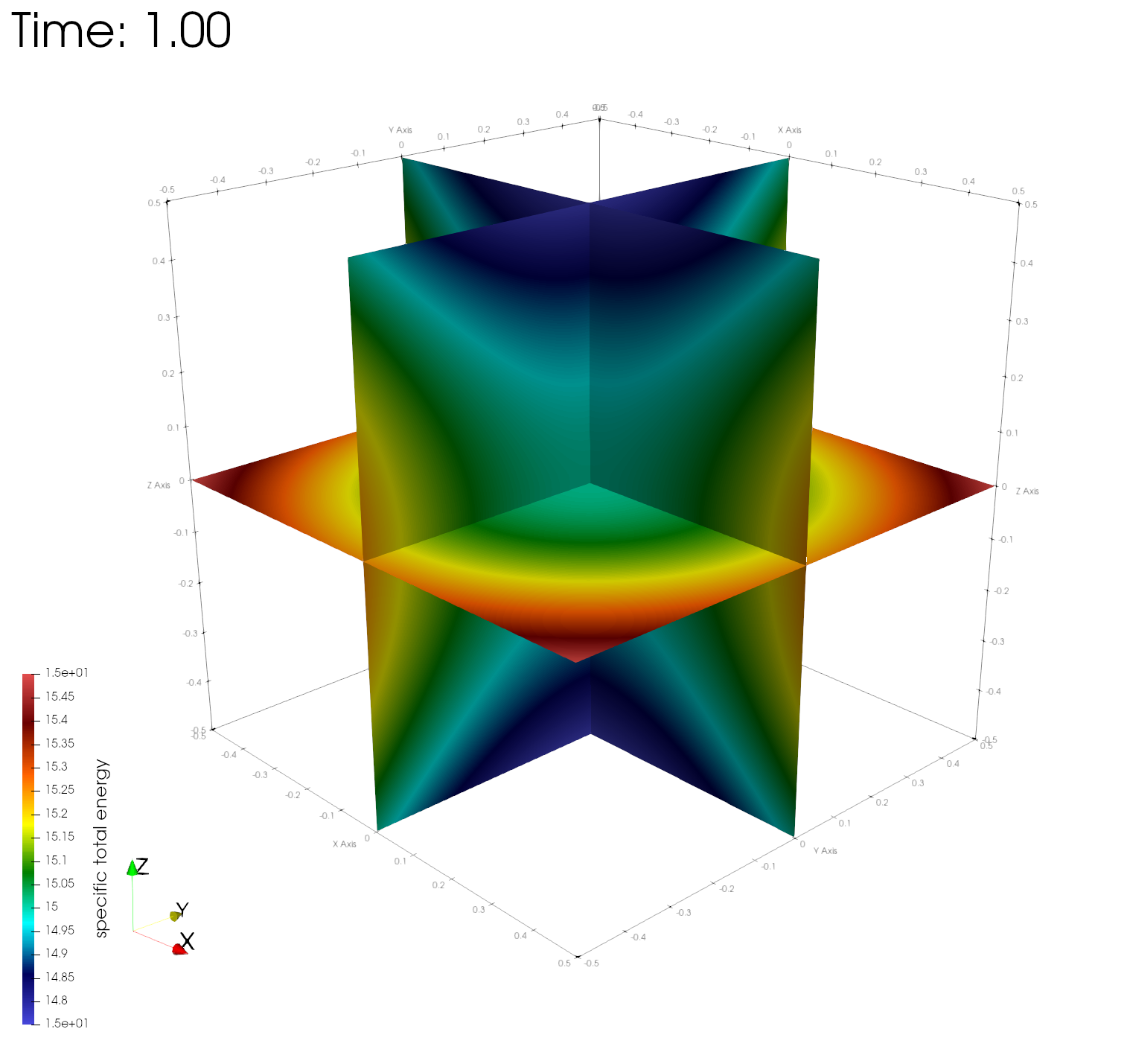
ParaView can be used for interactive visualization of the numerically computed fields as
paraview out.e-s.0.32.0The initial and final velocity, pressure, and total energy are depicted below.

Numerical errors
To estimate the order of convergence, the numerical solution is computed using three different meshes, whose properties of are tabulated below.
| Mesh | Points | Tetrahedra | h |
|---|---|---|---|
| 750K | 132,651 | 750,000 | 0.02 |
| 6M | 1,030,301 | 6,000,000 | 0.01 |
| 48M | 8,120,601 | 48,000,000 | 0.005 |
Here h is the average edge length. The next figure shows the time evolution of the L1 error in fluid density for the three different meshes. The L1 error is computed as
where n is the number of points, and are the exact and computed solutions at mesh point v, and denotes the volume associated to mesh point v.
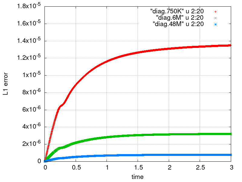
Gnuplot commands to reproduce the above plot:
set terminal png size 800,600 enhanced font "Helvetica,16"
set output "vortical_flow_L1r_kozcg.png"
set xlabel "time"
set ylabel "L1 error"
set grid
plot [] [:1.8e-5] "diag.750K" u 2:20, "diag.6M" u 2:20, "diag.48M" u 2:20
Convergence rate
The following table summarizes the L1 errors in all flow variables at the stationary state.
| Mesh | L1(r) | L1(u) | L1(v) | L1(w) | L(e) |
|---|---|---|---|---|---|
| 750K | 1.35e-5 | 2.41e-5 | 9.78e-6 | 1.05e-4 | 1.80e-4 |
| 6M | 3.21e-6 | 5.32e-6 | 1.47e-6 | 1.98e-5 | 4.18e-5 |
| 48M | 7.85e-7 | 1.29e-6 | 2.91e-7 | 3.32e-6 | 1.01e-5 |
| p | 2.03 | 2.04 | 2.34 | 2.57 | 2.05 |
Here r, u, v, w, and e are the fluid density, velocity in the x, y, z directions, and the internal energy, respectively. The order of convergence is estimated as
where m is a mesh index. As expected, the asymptotic convergence of the computed numerical solution in all variables approximates 2.
References
- J. Waltz and T.R. Canfield and N.R. Morgan and L.D. Risinger and J.G. Wohlbier, Manufactured solutions for the three-dimensional Euler equations with relevance to Inertial Confinement Fusion, Journal of Computational Physics, 267, 196–209, 2014.
- J. Waltz, T.R. Canfield, N.R. Morgan, L.D. Risinger, J.G. Wohlbier, Verification of a three-dimensional unstructured finite element method using analytic and manufactured solutions, Computers & Fluids, 81: 57-67, 2013.