V&V » LaxCG: Channel with a circular bump

This example uses LaxCG in Inciter to compute a stationary flow field in a channel with a circular bump on the lower wall at low and high Mach numbers.

This is a popular test problem, also known as Ni's test case. The problem consists of a channel with a circular bump in the bottom. The length of the channel is 3 units, its height is 1, and the width is 0.5. For the high-Mach-number case we set the inlet Mach number equal to 0.675 and for the low-Ma case to 0.001. Since the solution converges to steady state, the most efficient ways to compute this problem are to use implicit time marching or local time stepping [1] of which LaxCG implements the latter allowing taking larger time steps for larger cells.

Problem setup

The mesh, shown below, consists of 59,686 tetrahedra connecting 11,686 points. The initial conditions prescribe the Mach number of 0.675 and 0.001. At the inlet and outlet characteristic farfield boundary conditions are applied, while at the four sides symmetry (free-slip) boundary conditions are set.

Surface mesh for computing the transconic channel flow with a circular bump, nelem=60K, npoin=12K.

Code revision to reproduce

To reproduce the results below, use code revision 43ba64a and the control file below.

Control file

-- vim: filetype=lua:

print "Bump"

ttyi = 1000
cfl = 0.7

solver = "riecg"
--solver = "laxcg"

flux = "hllc"

steady = true
residual = 1.0e-14
rescomp = 1

part = "rcb"

mat = {
  spec_heat_ratio = 1.4
}

-- free stream
rho = 1.225
pre = 101325.0
mach = 0.675
--mach = 0.001
c = math.sqrt(mat.spec_heat_ratio * pre / rho)
print("Free-stream Mach number = ",mach)

ic = {
  density = rho,
  pressure = pre, 
  velocity = { c*mach, 0.0, 0.0 }
}

velinf = ic.velocity

bc_sym = {  
  sideset = { 3 }
}
         
bc_far = {
  density = ic.density,
  pressure = ic.pressure,
  velocity = ic.velocity,
  sideset = { 4 }
}

fieldout = {
  iter = 1000
}

diag = {
  iter = 10,
  format = "scientific",
  precision = 12
}

The solver and mach keywords above can be used to configure the solver and the Mach number.

Run on 32 CPUs

./charmrun +p32 Main/inciter -i bump.exo -c bump.q -r 100000

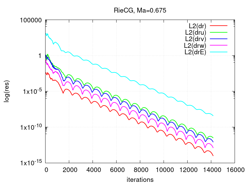
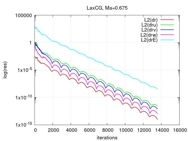
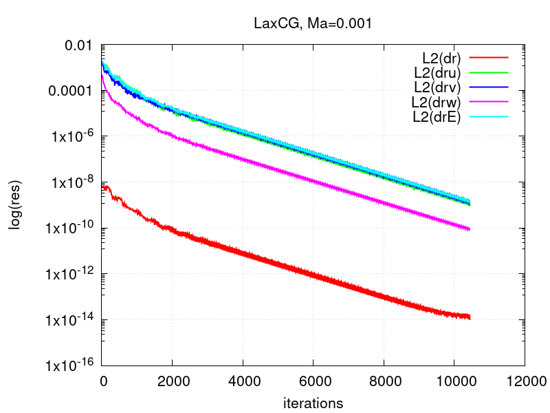
Convergence to steady state

The figures below depict the convergence history of the L2-norms of the residuals of the conserved quantities for the high-Ma case running RieCG and LaxCG, showing that both solvers converge.

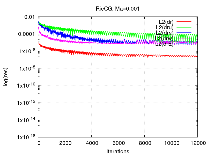
The next two figures show that computing the low-Ma case RieCG fails to converge, while the preconditioning facilitates convergence of the LaxCG solver.

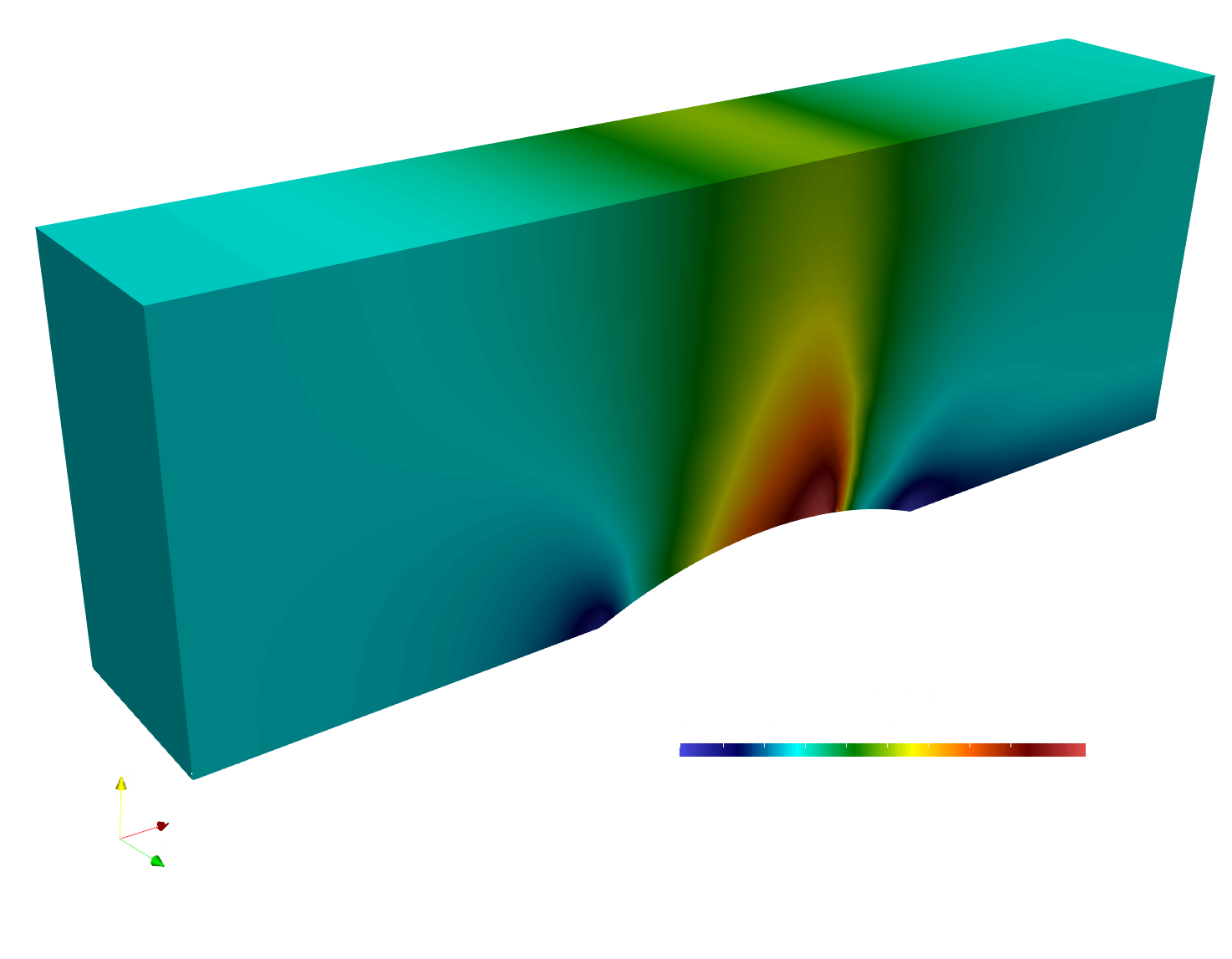
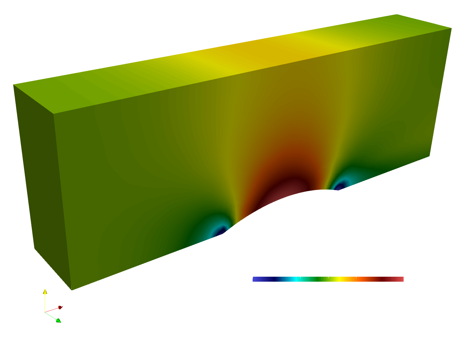
Visualization

ParaView can be used for interactive visualization of the numerically computed 3D fields as

paraview out.e-s.0.32.0

The converged Mach number distribution on the channel surface is depicted below, computed by the LaxCG solver for both Mach number configurations.

References

[1] R. Lohner, Applied Computational Fluid Dynamics Techniques: An Introduction Based on Finite Element Methods, Wiley, 2008.