V&V » LaxCG: Inviscid flow past a sphere

Problem configuration

The problem is configured with the free-stream Mach number of 0.001 to represent near-incompressible flow. Since the numerical solution converges to steady state, the most efficient ways to compute this problem are to use implicit time marching or local time stepping [1] of which the latter is implemented in LaxCG allowing larger time steps for larger cells.

Problem setup

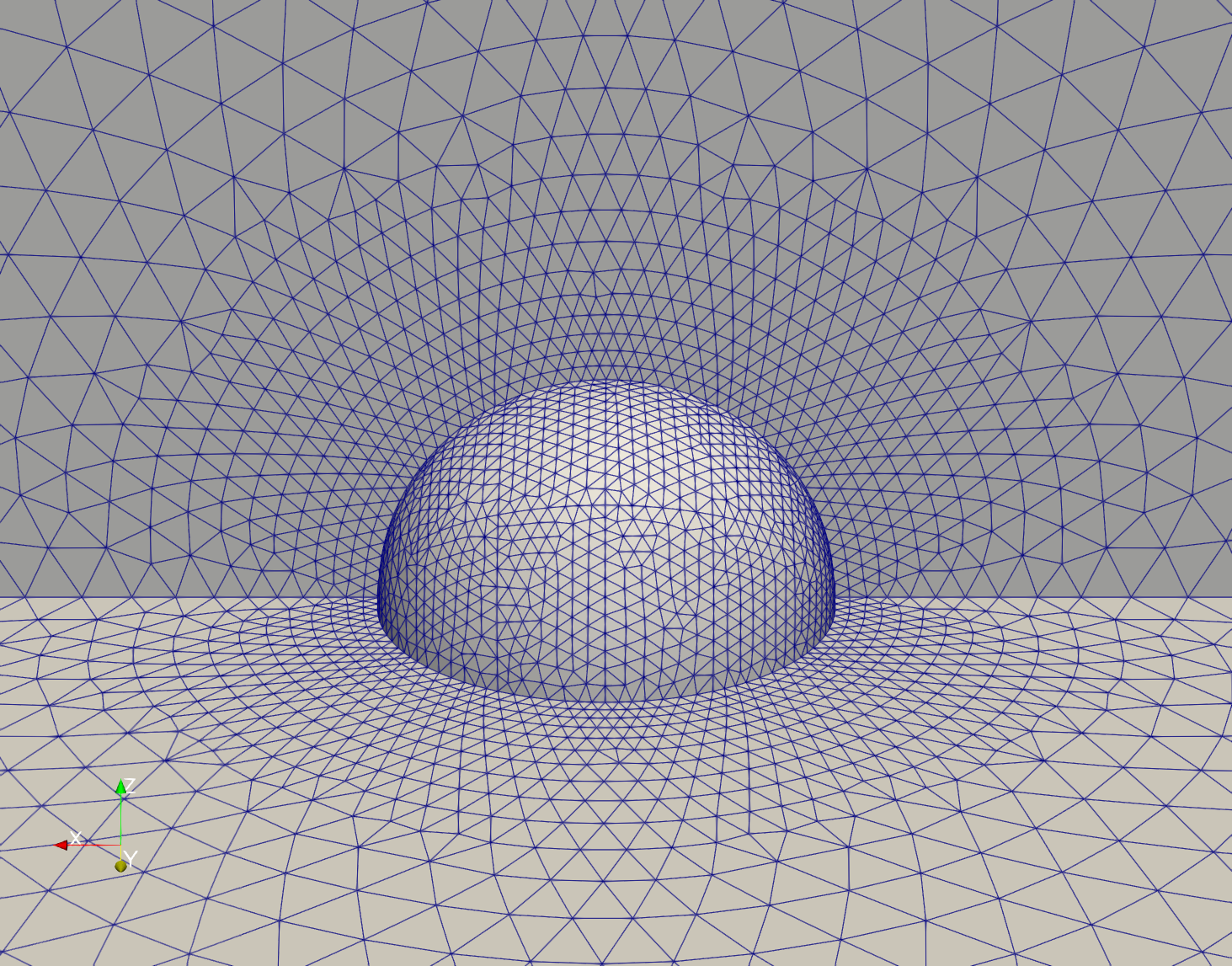
Due to the spatial symmetry of the problem, only quarter of the sphere is represented. The computational mesh consists of 73,397 tetrahedra connecting 14,281 points, whose surface mesh is depicted below. The initial conditions prescribe the free-stream Mach number and the flow variables are non-dimensionalized and parameterized by this quantity to yield unit streamwise velocity in the X direction. Symmetry (free-slip) conditions are applied on the sphere and the symmetry surfaces, while characteristic far-field boundary conditions are applied on the rest of the domain boundary.

Code revision to reproduce

To reproduce the results below, use code revision 43ba64a and the control file below.

Control file

-- vim: filetype=lua:

print "Sphere"

nstep = 12000
ttyi = 1000
cfl = 0.7

solver = "laxcg"
flux = "hllc"

steady = true
residual = 1.0e-14
rescomp = 2

part = "phg"

mat = {
  spec_heat_ratio = 1.4
}

-- free stream
mach = 0.001
print("Free-stream Mach number = ",mach)

ic = {
  density = 1.0,
  pressure = 1.0 / mach / mach / mat.spec_heat_ratio,
  velocity = { 1.0, 0.0, 0.0 }
}

velinf = ic.velocity

bc_sym = {
  sideset = { 1, 2, 3 }
}

bc_far = {
  density = ic.density,
  pressure = ic.pressure,
  velocity = ic.velocity,
  sideset = { 4, 5, 6, 7 }
}

fieldout = {
  iter = 10000,
  sideset = { 1, 2, 3 }
}

diag = {
  iter = 10,
  format = "scientific",
  precision = 12
}

Run using 32 CPUs

./charmrun +p32 Main/inciter -i sphere.exo -c sphere.q

Visualization

ParaView can be used for interactive visualization of the numerically computed 3D fields as

paraview out.e-s.0.32.0

Results only on the symmetry surfaces can be visualized by first stitching the partitioned surface output files into single surface output files, then loading them all into paraview:

Main/meshconv -i out-surf.1.e-s.0.32.% -o out-surf.1.exo
Main/meshconv -i out-surf.2.e-s.0.32.% -o out-surf.2.exo
Main/meshconv -i out-surf.3.e-s.0.32.% -o out-surf.3.exo

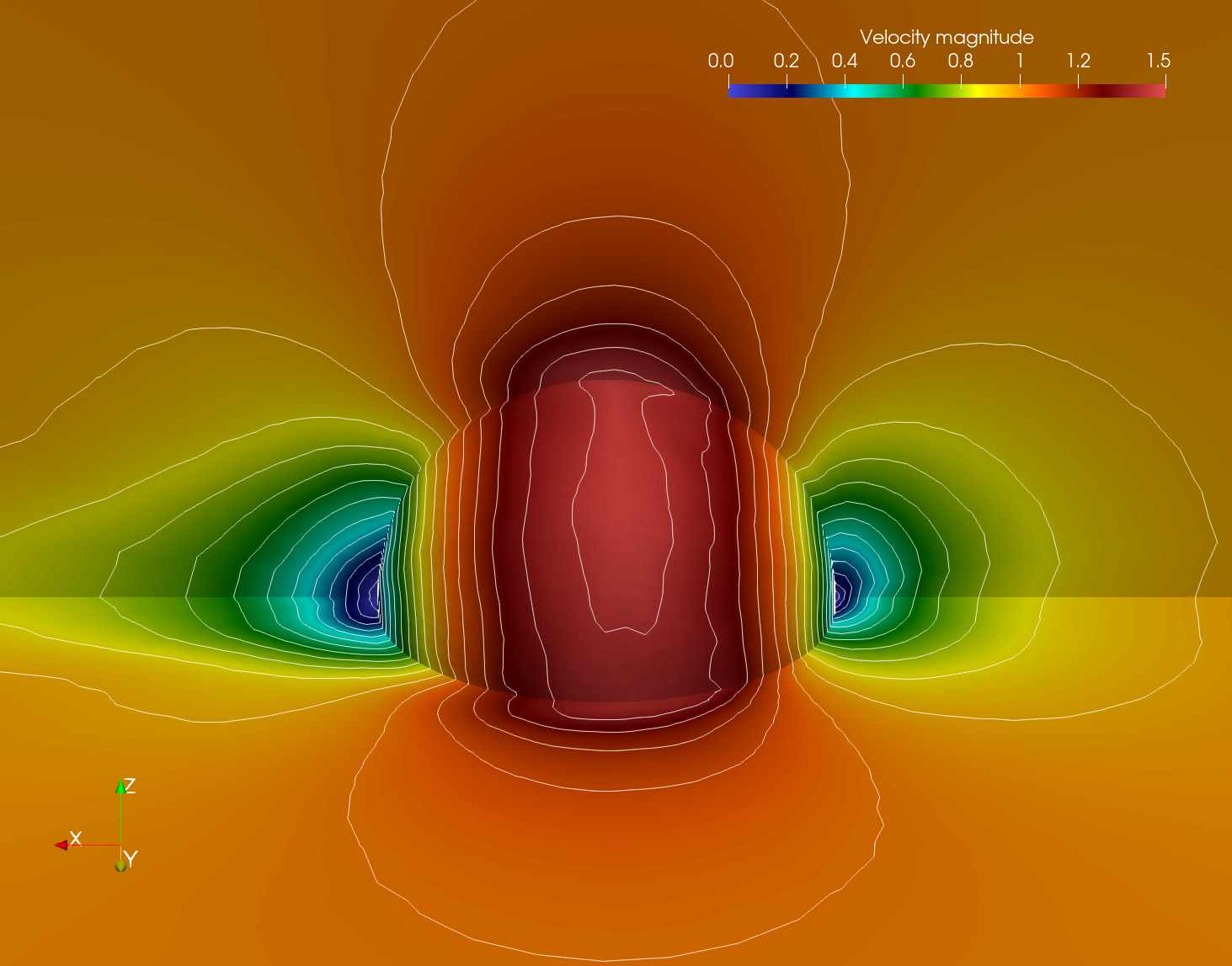
The velocity magnitude on the sphere and symmetry surfaces is depicted below, computed by the LaxCG solver.

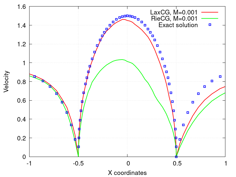
The velocity magnitude extracted along the centerline and the sphere surface is depicted below computed by LaxCG. Also plotted is the analytic solution from potential flow theory and the solution produced by RieCG. As the figure shows the time-derivative preconditioning implemented in LaxCG produces a superior solution to RieCG without preconditioning.

References

- R. Lohner, Applied Computational Fluid Dynamics Techniques: An Introduction Based on Finite Element Methods, Wiley, 2008.