LohCG: Dispersion from a point source in shear flow
This example uses LohCG in Inciter to compute a problem featuring advection, shear, and diffusion of a passive scalar. Since the analytic solution is known as a function of time, numerical errors can be estimated. This enables quantifying the accuracy of the numerical method as well as verifying the correctness of the implementation.
Equations solved
In this example we numerically solve the linear advection equation of a passive scalar, denoted by , representing the normalized concentration of a pollutant released from a concentrated source, coupled to the Navier-Stokes equations governing viscous Newtonian constant-density flow, see also LohCG, as
where is the (constant) speed of sound, is the velocity vector, is the pressure, and both the pressure and the viscosity have been normalized by the (constant) density. Here is the scalar diffusivity. Furthermore, , is a source term that arises from the prescribing a known velocity field, used for verification only, specified below. This source term is zero when computing practical engineering problems.
Problem setup
This problem and its analytical solution was presented by Carter and Obuko [1] with further related discussion in [2]. For the simple steady two dimensional uni-directional flow, with velocity along the axis, shear and constant diffusion coefficient, , the governing equation is
subject to initial conditions
When the initial condition is a point source of mass at , the solution is
To allow the numerical solution to be based on a finite source size, the calculation is started at time with a concentration distribution given by the above analytic solution using , i.e., the initial concentration peak is unity. The problem is solved on a 3D rectangular domain with a few cells in the dimension and extents with , , , , and .
While we are only interested in the evolution of the scalar, we prescribe the source term that yields a stationary flow with a prescribed translational and sheared velocity field as
The initial conditions are sampled from the analytic solutions above. We set inhomogeneous Dirichlet boundary conditions for all variables on the sides of the domain with normals in the or directions, sampling their analytic solutions. On the sides with normals in the direction, the flow variables are sampled from their analytic solutions, while for the scalar, homogeneous Neumann conditions are enforced.
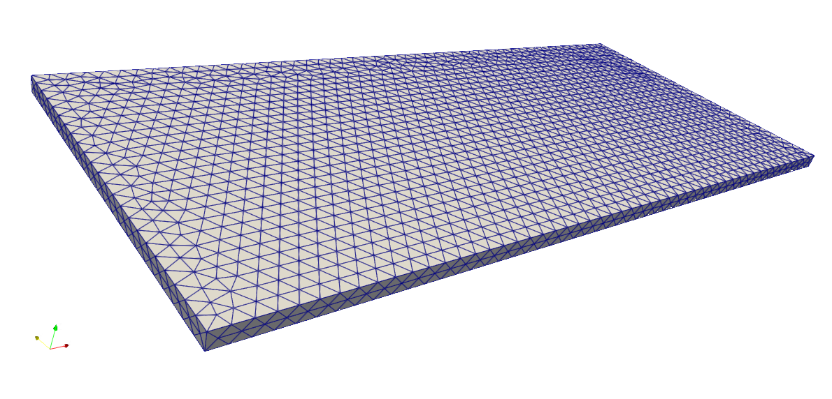 Coarse surface mesh for computing the shear-diffusion test problem, nelem=15K, npoin=3K.
Code revision to reproduce
To reproduce the results below, use code revision 8c88d03 and the control file below.
Control file
-- vim: filetype=lua:

print "2D shear-diffusion"

-- mesh: shear_15K.exo
--       shear_124K.exo

t0 = 2400.0
term = 9600.0
ttyi = 100

cfl = 0.3

solver = "lohcg"
flux = "damp4"
rk = 4
soundspeed = 10.0

part = "rcb"

problem = {
  name = "sheardiff",
  p0 = 0.5,             -- x translation velocity (u_0)
  alpha = 1.0e-4        -- y shear velocity (lambda)
}

mat = {
  dyn_diffusivity = 50.0
}

pressure = {
  iter = 1,
  tol = 1.0e-3,
  pc = "jacobi",
  hydrostat = 0
}

bc_dir = {
  { 1, 0, 1, 1, 1, 1 },
  { 2, 0, 1, 1, 1, 0 }
}

fieldout = {
  iter = 100
}

diag = {
  iter = 1,
  format = "scientific",
  precision = 12
}
Run using on 32 CPUs
./charmrun +p32 Main/inciter -i shear_124K.exo -c sheardiff_lohcg.q
Visualization
ParaView can be used for interactive visualization of the numerically computed fields as
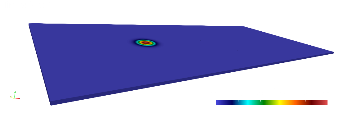
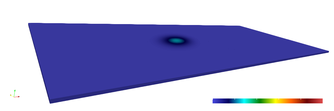
paraview out.e-s.0.32.0The scalar field is displayed at the initial and final times below.
Numerical solutions and errors
To estimate the order of convergence, the numerical solution was computed using two different meshes, whose properties of are tabulated below.
| Mesh | Points | Tetrahedra | h |
|---|---|---|---|
| 1 | 3,134 | 9,123 | 640.99 |
| 2 | 24,992 | 74,156 | 218.97 |
Here h is the average edge length. The L1 and L2 errors are computed as
where is the total number of points in the whole domain, and are the exact and computed scalar concentrations at mesh point , and denotes the volume associated to mesh point . The table below displays the numerical errors for the two meshes and the estimated order of convergence, computed by
where is a mesh index.
| Mesh | h | L1(err) | L2(err) |
|---|---|---|---|
| 1 | 640.99 | 6.486e-04 | 3.697e-03 |
| 2 | 218.97 | 5.825e-05 | 3.357e-04 |
| p | 2.244 | 2.234 |
References
- H. Carter, A. Okubo, A study of the physical processes of movement and dispersion in the Cape Kennedy area, Chesapeake Bay Inst. Ref. 65-2, Johns Hopkins Univ., 1965.
- A. Okubo, M. Karweit, Diffusion from a continuous source in a uniform shear flow, Limm. and Oceano. 14(4) 514-520., 1969.