RieCG: Sod's shocktube
This example uses RieCG in Inciter to compute the Sod problem [1], widely used to test numerical methods to model discontinuous solutions. The problem consists of a pipe in which two different states of a gas is initially separated by a diaphragm. When the diaphragm is raptured at t=0, a wave structure is created and propagated in time. While the solution is 1D, we modeled the process in 3D. The available analytic solution enables verification of the accuracy of the numerical method and the correctness of the software implementation.
Equations solved
The system of equation solved is
detailed at the RieCG page describing its numerical method.
Problem setup
The problem is modeled as a 3D tube with a circular cross section of unit length with a diameter of 0.05, with the specific heat ratio as 1.4, and the following initial conditions
where is the distance along the length of the tube. Dirichlet boundary conditions were applied on all flow variables sampling their initial values at the end-faces of the domain and symmetry (free-slip) conditions were set along the surface of the tube. The numerical solution was advanced using the CFL number 0.5 using four different meshes whose properties are list in the following table:
| Mesh | Points | Tetrahedra | h |
|---|---|---|---|
| 0 | 7,294 | 34,181 | 0.008393 |
| 1 | 51,794 | 273,448 | 0.004138 |
| 2 | 389,139 | 2,187,584 | 0.002060 |
| 3 | 3,014,277 | 17,500,672 | 0.001028 |
Here h is the average edge length along the length of the tube.
Code revision to reproduce
To reproduce the results below, use code revision 965089c and the control file below.
Control file
-- vim: filetype=lua:

print "Sod shocktube"

term = 0.2
ttyi = 10
cfl = 0.5

part = "rcb"

problem = {
  name = "sod"
}

mat = { spec_heat_ratio = 1.4 }

bc_sym = {
  sideset = { 2 }
}

bc_dir = {
 { 1, 1, 1, 1, 1, 1 },
 { 3, 1, 1, 1, 1, 1 }
}

fieldout = {
  iter = 10000
}

diag = {
  iter = 1,
  format = "scientific"
}
Run using mesh 1 on 4 CPUs
./charmrun +p4 Main/inciter -i tube01.exo -c sod.q
Visualization
ParaView can be used for interactive visualization of the numerically computed fields as
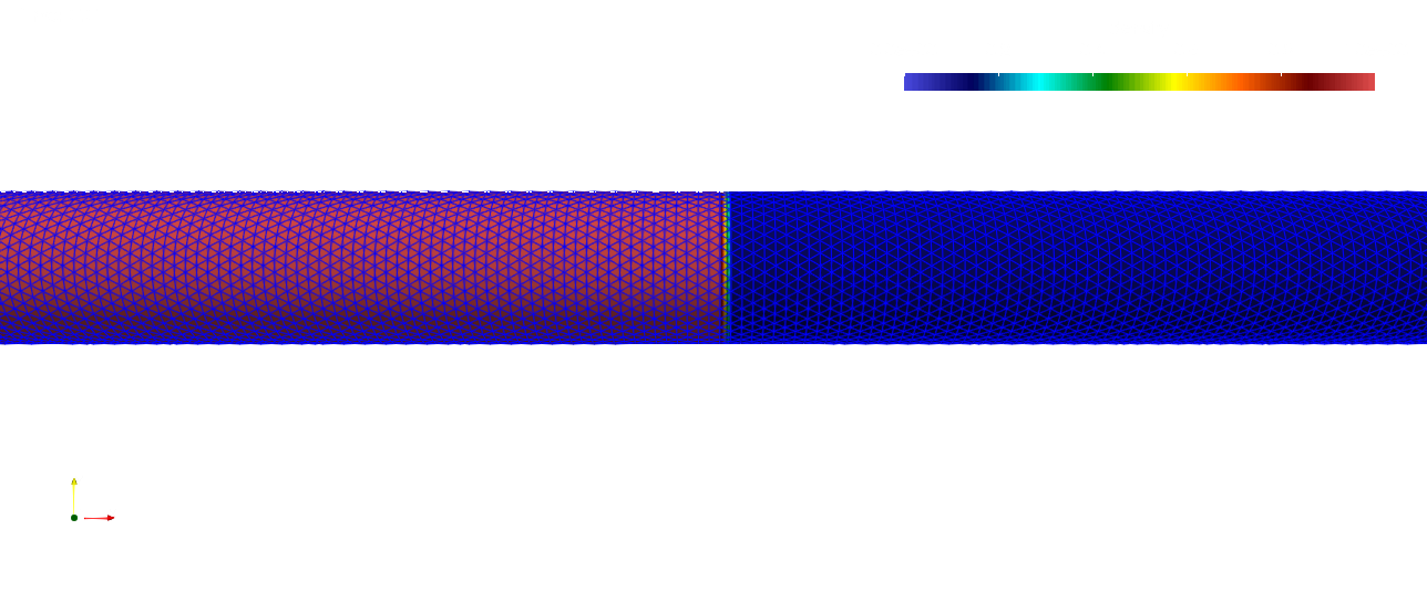
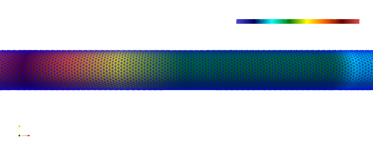
paraview out.e-s.0.4.0The surface mesh colored by the fluid density at t=0 and t=0.2 on mesh 1 are depicted below.
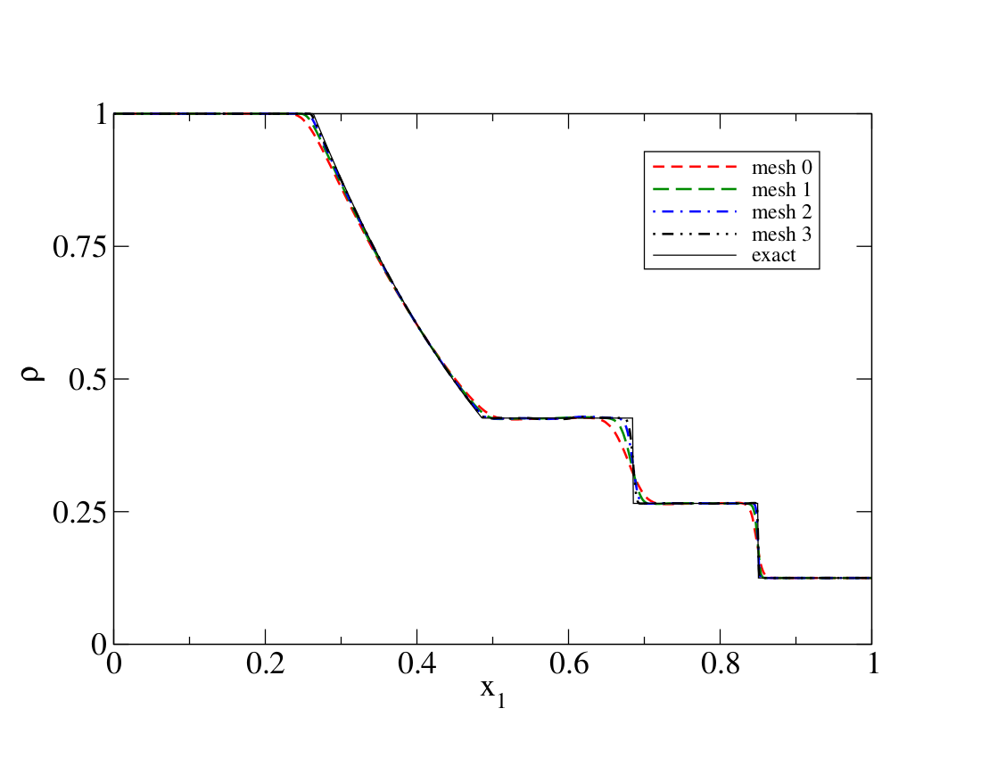
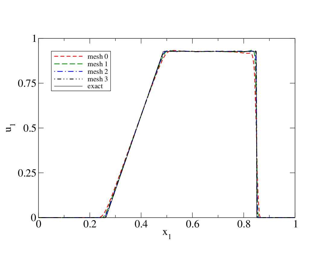
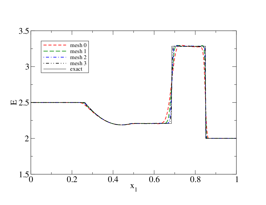
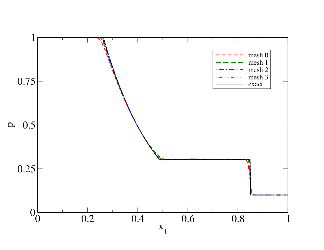
The numerical solution is also extracted at t=0.2 along the center of the tube. The density, velocity, total energy, and pressure are depicted below for the successively finer meshes together with the analytical solution.
Numerical errors and convergence rate
The table below shows the numerical L1 errors of the flow quantities computed. The L1 error is computed as
where n is the total number of points of the mesh, and are the exact and computed solutions at mesh point v, and denotes the volume associated to mesh point v. The order of convergence is estimated as
where m is a mesh index. The following table summarizes the L1 errors in all flow variables at t=0.2.
| Mesh | h | L1(r) | L1(u) | L1(p) | L1(E) |
|---|---|---|---|---|---|
| 0 | 0.008393 | 6.14e-3 | 1.01e-2 | 4.82e-3 | 2.47e-2 |
| 1 | 0.004138 | 3.53e-3 | 5.24e-3 | 2.77e-3 | 1.38e-2 |
| 2 | 0.002060 | 2.12e-3 | 2.79e-3 | 1.67e-3 | 8.12e-3 |
| 3 | 0.001028 | 1.31e-3 | 1.67e-3 | 1.05e-3 | 4.88e-3 |
| p | 0.69 | 0.73 | 0.67 | 0.73 |
Here r, u, p, and E are the fluid density, velocity along the tube, pressure, and total energy, respectively. The data is also plotted in the folloowing figure
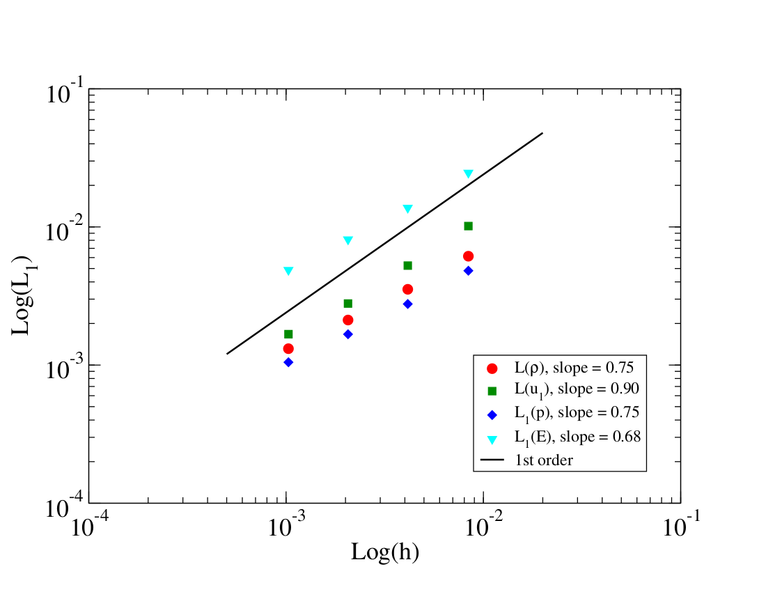
Since the solution contains discontinuities, the error is dominated by their vicinity and thus the order of accuracy is expected to be approximately 1.0 or lower.
References
- J.R. Kamm, Enhanced verification test suite for phyics simulation codes, LA-14379, SAND2008-7813, 2008.