RieCG: Square cavity
This example uses RieCG in Inciter to a perform a numerical study of the interaction of a planar shock wave with a square cavity. The computed numerical results are compared to the experimental data published in [1].
Shock wave diffractions arise in a number of practical applications. An example is internal combustion engines, where inflow/outflow valves are periodically opened and shut in a dynamic fashion, giving rise to waves, which then interact with the cylinder walls. Another example is building vulnerability assessments to air blasts. Important engineering features predicted from such simulations are wave structures and the resulting pressure-load time-histories in various locations of the complex geometries of the simulation domains. Such time-dependent problems test the ability of numerical methods for compressible flows to accurately propagate waves at distances as well as the accuracy of complex wave interaction patterns.
Problem setup
The problem setup is illustrated in the following figure:
A planar shock wave is created by two disparate states separated by a diaphragm. Removing the diaphragm at time t=0 produces a shock wave, moving toward the square cavity which produces an elaborate interaction with shocks reflected from the cavity walls. The initial state at t=0 correspond to Ms=1.3 in [1] as
Since the problem is 2D, the computational domain consists of a single cell in the z direction. Characteristic boundary conditions are applied at the left side of State 2 and symmetry (free-slip) conditions are set at walls. The numerical simulations are also instrumented to record time histories of the pressure in time at the 3 gauge locations depicted in the figure above.
Code revision to reproduce
To reproduce the results below, use code revision 7b4edaf and the control file below.
Control file
-- vim: filetype=lua:

print "Square cavity"
print [[Igra, Falcovitz, Reichenbach, Heilig, 'Experimental and
        numerical study of the interaction between a planar shock
        wave and a square cavity', Journal of Fluid Mechanics, 313,
        105-130, 1996.]]

term = 200.0
ttyi = 100
cfl = 0.5

solver = "riecg"
part = "rcb"

mat = { spec_heat_ratio = 1.407 }

ic = { -- bg: state 2
  density = 1.689e-3,
  pressure = 1.753e-6,
  velocity = { 0.01544, 0.0, 0.0 },
  boxes = { -- state 0
    { x = { 4.35, 20.5 },
      y = { -0.5, 12.0 },
      z = { -0.5, 0.5 },
      density = 1.1155e-3,
      pressure = 0.96e-6,
      velocity = { 0, 0, 0 }
    }
  }
}

bc_sym = {
  sideset = { 1, 2 }
}

bc_far = { -- inflow (state 2)
  density = 1.689e-3,
  pressure = 1.753e-6,
  velocity = { 0.01544, 0.0, 0.0 },
  sideset = { 3 }
}

fieldout = {
  iter = 100,
  time = 20.0
}

histout = {
  iter = 1,
  points = {
    { 5.01, 2.5, 0.01 },
    { 7.5, 0.01, 0.01 },
    { 9.99, 2.5, 0.01 }
  }
}

diag = {
  iter = 1,
  format = "scientific"
}
Run on 4 CPUs
./charmrun +p4 Main/inciter -i squarecav_100K.exo -c squarecav.q
Visualization
ParaView can be used for interactive visualization of the numerically computed 3D fields as
paraview out.e-s.0.4.0Time-evolution of pressure
The figure below depicts the computed pressure field together with a shadowgraph taken from the experiments at t=200us. It is clear from the figure, that the unique wave pattern of primary and reflected shocks as well as a vortex forming at the upper-left corner of the cavity are all accurately reproduced by the numerical simulation. Excellent agreement can be found between the curvature, the geometry, and the location of the computed wave patterns and the experimental data. For more a detailed discussion of the process with more snapshots in time, see Papers.
Mesh sensitivity
To investigate the effect of mesh resolution, we simulated the problem using 4 different meshes listed in the following table.
| Mesh | Points | Tetrahedra | h |
|---|---|---|---|
| 0 | 33,983 | 100,620 | 0.0911 |
| 1 | 138,518 | 423,826 | 0.0475 |
| 2 | 545,982 | 1,664,333 | 0.0268 |
Here h is the average edge length.
The following figures show the computed fluid density fields at t=200us from the calculations using mesh 0 and 2.
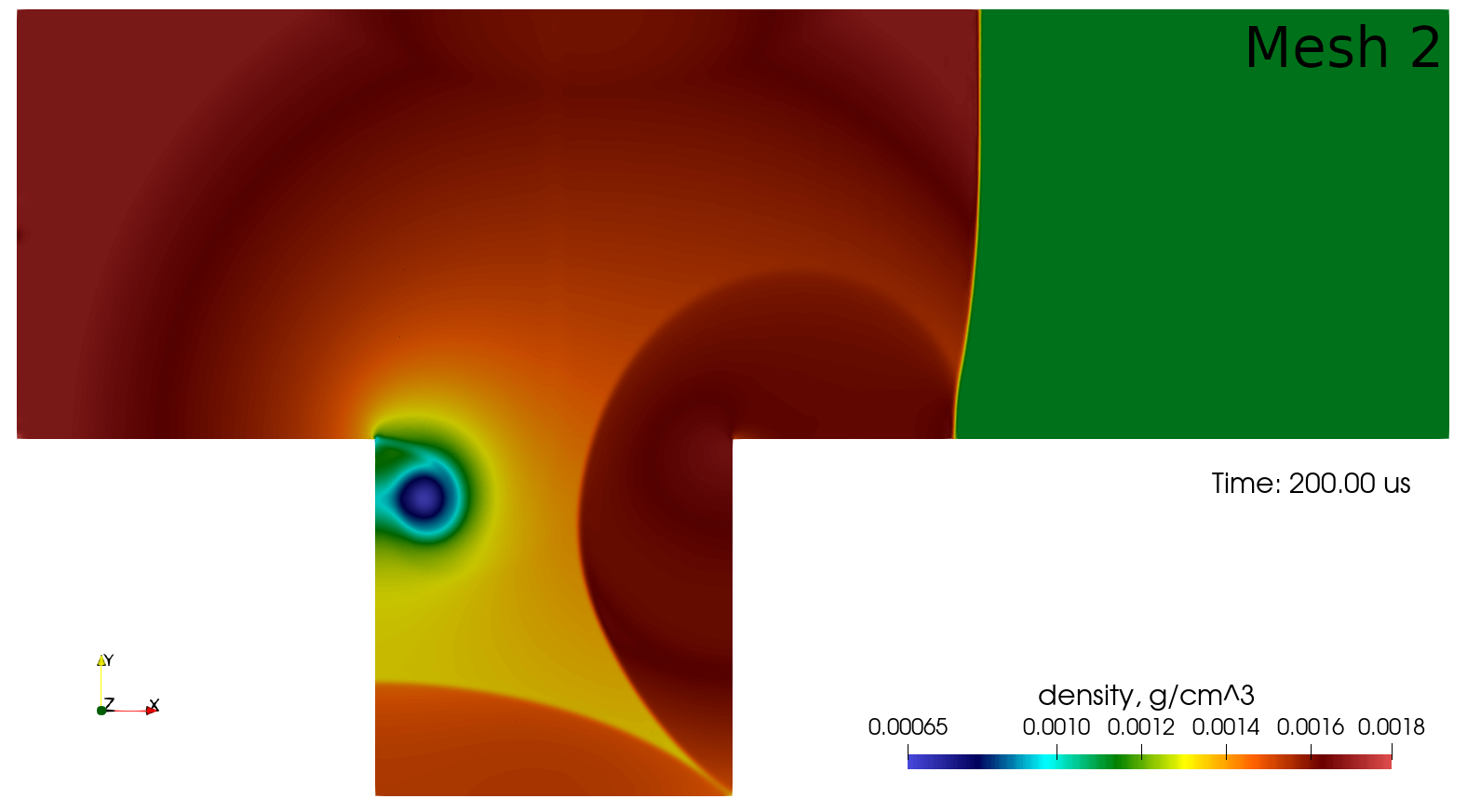
As expected, increasing the mesh resolution yields sharper resolution of the shocks and diffuses the vortex, however, due to the conservative nature of the numerical scheme, the predicted locations of the shocks do not change with mesh refinement.
Pressure time-histories
The figure below depicts the evolution of the pressure time-histories recorded from the numerical simulations at the 3 gauges depicted in the problem setup. The pressure histories are displayed from the calculations using Meshes 0 and 2. The pressure values are normalized by the pre-shock pressure, p_0.
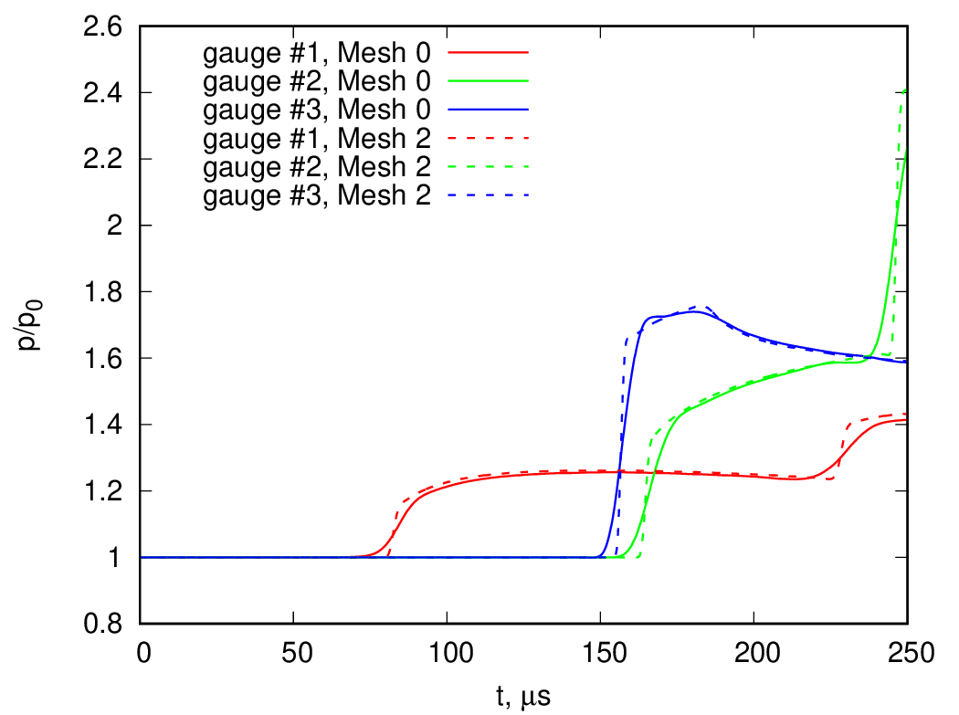
It is evident that mesh resolution does not significantly change the numerical pressure gauge readouts, only the temporal gradients become sharper with increased resolution. The first pressure peaks, the highest pressures encountered at the walls when a shock first hits them, are available from the experiments, and compared to those obtained from the numerical simulations in the table below.
| Gauge | Experiment | Computation | Error |
|---|---|---|---|
| #0 | 1.25 | 1.26 | -0.79% |
| #1 | 1.51 | 1.58 | -4.64% |
| #2 | 1.77 | 1.76 | 0.57% |
The errors in the last column are computed by
where p_s is the first peak in the pressure and p_0 is the pre-shock pressure. Again, there is excellent agreement between the experimental and computed data.
References
- O. Igra, J. Falcovitz, H. Reichenbach, W. Heilig, Experimental and numerical study of the interaction between a planar shock wave and a square cavity, J. Fluid Mech. 313., 105-130, 1996.