Examples » ZalCG: F16

This example uses ZalCG in Inciter to compute the stationary flow field around an F-16 fighter jet.

The test case is configured with the Mach number of 0.84 and an angle of attack of 3.06 degrees, which yields a transonic flow. Since the solution converges to steady state, the most efficient ways to compute this problem are to use implicit time marching or local time stepping [1] of which ZalCG implements the latter allowing taking larger time steps for larger cells.

Problem setup

The mesh, shown below, consists of 6,028,542 tetrahedra connecting 1,042,051 points. The initial conditions prescribe the Mach number of 0.84 and the velocity with an angle of attack of 3.06 degrees. At the outer surface of the domain characteristic far-field boundary conditions are applied while symmetry (free-slip) conditions are applied on the airplane body.

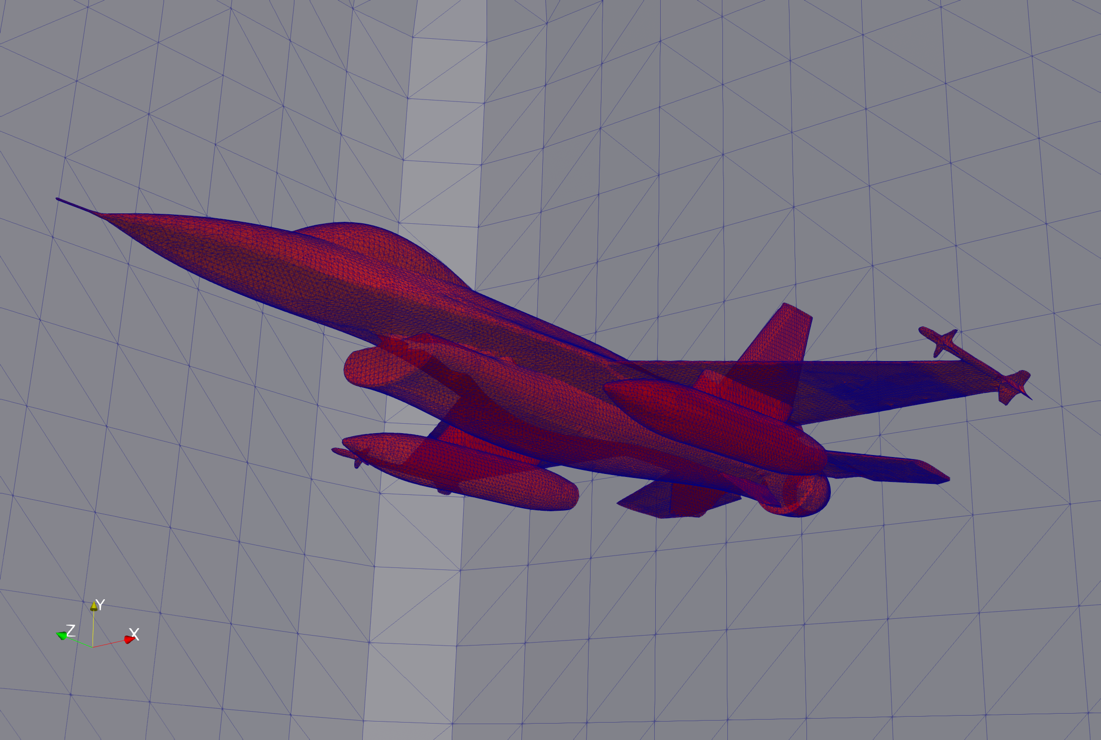Surface mesh for computing the flow around the F-16, nelem=6M, npoin=1M.

Code revision to reproduce

To reproduce the results below, use code revision feda946 and the control file below.

Control file

-- vim: filetype=lua:

print "F16 in steady transconic flow"

ttyi = 100
cfl = 0.3

solver = "zalcg"
fct = false
stab2 = true
stab2coef = 0.2

nstep = 2000
steady = true
rescomp = 1

part = "phg"

mat = { spec_heat_ratio = 1.4 }

rho = 1.225     -- density of air at STP, kg/m3
pre = 1.0e+5    -- N/m^2
mach = 0.84     -- free stream Mach number
angle = 3.06    -- angle of attack

-- free stream sound speed
a = math.sqrt( mat.spec_heat_ratio * pre / rho )

ic = {
  density = rho,
  pressure = pre,
  velocity = { 0.0,
               mach * a * math.sin(angle*math.pi/180.0),
              -mach * a * math.cos(angle*math.pi/180.0) }
}

bc_sym = {
  sideset = { 1 }
}

bc_far = {
  density = rho,
  pressure = pre,
  velocity = ic.velocity,
  sideset = { 12 }
}

fieldout = {
  iter = 1000,
  sideset = { 1 }
}

diag = {
  iter = 10,
  format = "scientific",
  precision = 12
}

Run using on 32 CPUs

./charmrun +p32 Main/inciter -i f16b_tet.exo -c f16.q |& tee f16.out

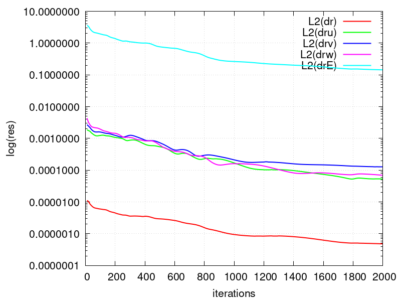
Convergence to steady state

The figure below shows the convergence history of the L2-norms of the residuals of the conserved quantities.

Visualization

ParaView can be used for interactive visualization of the numerically computed 3D fields as

paraview out.e-s.0.32.0

Results on the airplane body and symmetry surfaces can be visualized by first stitching the partitioned surface output files into a single surface output file followed by invoking paraview on the stitched surface exo file:

Main/meshconv -i out-surf.1.e-s.0.32.% -o out-surf.1.exo
paraview out-surf.1.exo

The Mach number distribution on the airplane body and symmetry surface is depicted below from different angles.

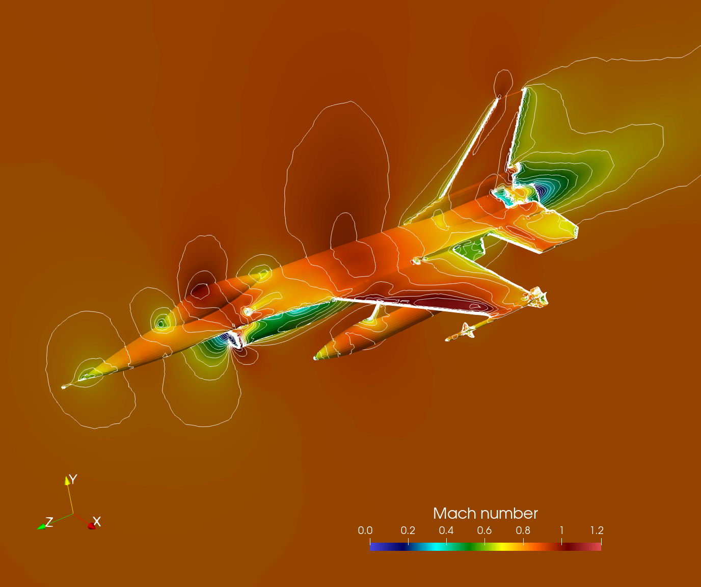
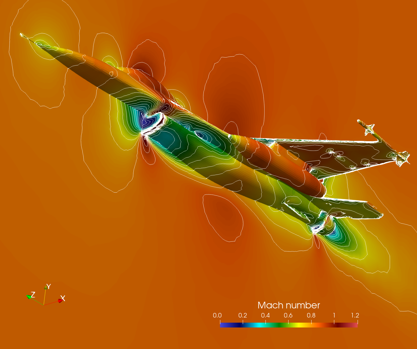Mach number distribution and contours on the airplane body and symmetry plane.

References

[1] R. Lohner, Applied Computational Fluid Dynamics Techniques: An Introduction Based on Finite Element Methods, Wiley, 2008.