ZalCG: Urban-scale pollution from a point source
This example uses ZalCG in Inciter to compute pollution released from a point source in an urban environment. The goal is to demonstrate basic capability of the flow solver in ZalCG coupled to atmospheric dispersion of a passive scalar that can represent pollution concentration.
Equations solved
In this example we solve the Euler equations coupled to a scalar, representing pollutant concentration, as
where the summation convention on repeated indices has been applied, is the density, is the velocity vector, is the specific total energy, is the specific internal energy, and is the pressure, while denotes the concentration of pollution normalized by its value at the source. The system is closed with the ideal gas law equation of state
where is the ratio of specific heats.
Problem setup
We configure the ZalCG solver to compute an urban-scale pollution problem in a typical city whose computational domain contains many of the buildings in downtown Győr, located in North-West of Hungary. The surface mesh is displayed with some of its characteristics in the table below.
| Dimensions, km | h, m | Points | Tetrahedra |
|---|---|---|---|
| 9.2 x 6.7 x 1.5 | 11.3 | 1,746,029 | 10,058,445 |
Here h is the average edge length.
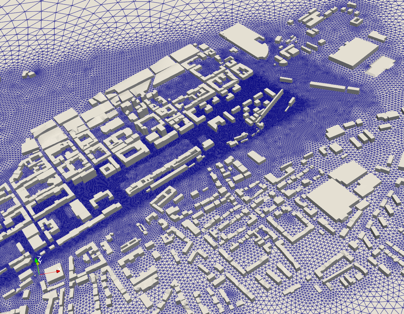 Surface mesh for computing an urban-scale pollutatnt dispersion study in the Hungarianc city of Győr.
Initial conditions are specified by atmospheric conditions at sea level at 15C as
and these conditions are also enforced as Dirichlet boundary conditions on the top and sides of the brick-shaped domain during time stepping.
The scalar, , representing pollutant concentration is released from a point source at t=10s of the 140s total time simulated. The value of the scalar is normalized to the constant value of c=1.0 at the source. After verifying that the norms of the velocity component residuals decrease at least two orders in magnitude from their initial values, the flow is assumed to be stationary, the numerical values of density, momentum, and total energy are no longer updated, and the scalar is released.
Code revision to reproduce
To reproduce the results below, use code revision 77cba43f and the control file below.
Control file
-- vim: filetype=lua:

print "Urban-scale pollution"

-- meshes:
-- gyor_m1_10M.exo

scalar_release_time = 10.0

term = 140.0

ttyi = 10
cfl = 0.9

part = "phg"

solver = "zalcg"
stab2 = true
stab2coef = 0.2

freezetime = 10.0
freezeflow = 4.0

problem = {
  name = "point_src",
  src = {
    location = { 1914.0, 1338.0, 20.0 },
    radius = 10.0,
    release_time = scalar_release_time
  }
}

mat = { spec_heat_ratio = 1.4 }

ic = {
  density = 1.225,
  pressure = 1.0e+5,
  velocity = { -10.0, -10.0, 0.0 }
}

bc_dir = {
  { 1, 1, 1, 1, 1, 1, 0 },
  { 9, 1, 1, 1, 1, 1, 0 }
}

bc_sym = {
  sideset = { 10, 21, 22, 23, 24 }
}

fieldout = {
  iter = 100,
  time = 10.0,
  sideset = { 10, 21, 22, 23, 24 },
  --range = {
  --  { scalar_release_time, term, 10.0 }
  --}
}

diag = {
  iter = 10
}
Run on 128 CPU cores in Charm++'s non-SMP mode using SLURM
srun --nodes=1 --ntasks-per-node=128 Main/inciter -c gyor3nodea.q -i gyor_m1_10M.exo
Visualization
ParaView can be used for interactive visualization of the numerically computed 3D fields as
paraview out.e-s.0.128.0Results only on the ground and building surfaces can be visualized by first stitching the partitioned surface output files into single surface output files (one for each surface) followed by invoking paraview on the stitched surface exo files:
for i in 10 21 22 23 24; do Main/meshconv -i out-surf.$i.e-s.0.128.% -o out-surf.$i.exo; done
paraview --data="out-surf.10.exo;out-surf.21.exo;out-surf.22.exo;out-surf.23.exo;out-surf.24.exo"
Pollution concentration snapshot
The figure below depicts ground-level concentrations at t=90s.
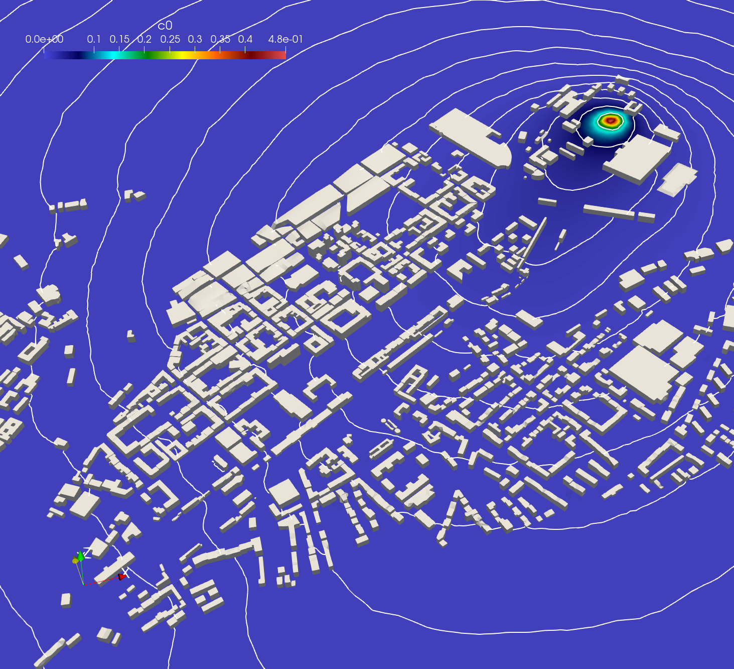 Surface distributions of a propagating scalar representing pollutant concentration in an urban-scale air quality study with stationary winds, computed on 128 CPUs.