ZalCG: ONERA wing
This example uses ZalCG in Inciter to demonstrate and validate the solver in a 3D complex-geometry case by comparing the numerical results to experimental data.
We computed the popular and well-documented aerodynamic flow over the ONERA M6 wing, see e.g., [1]. The available experimental data of the pressure distribution along the wing allows validation of the numerical method. The problem is configured with a Mach number of 0.84 and an angle of attack of 3.06 degrees, which yields a transonic flow. Since the solution converges to steady state, the most efficient ways to compute this problem are to use implicit time marching or local time stepping [2] of which ZalCG implements the latter allowing taking larger time steps for larger cells.
Problem setup
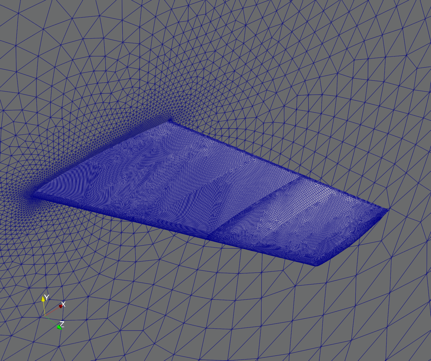
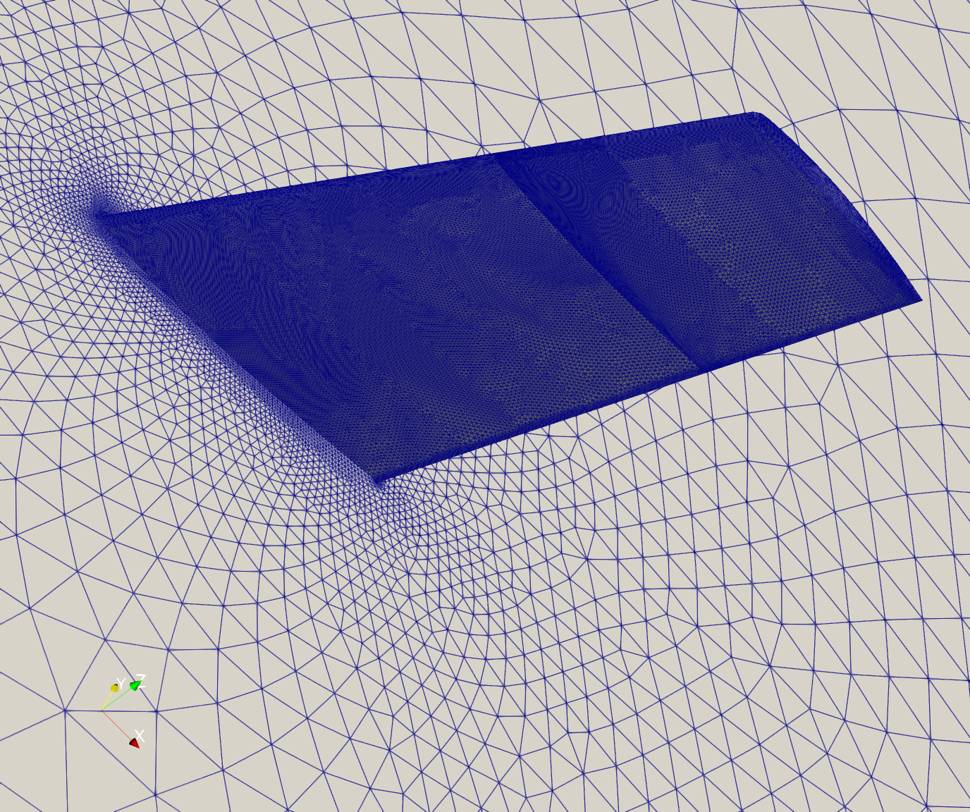
We used a coarser and a finer computational mesh whose properties are displayed below.
| Mesh | Points | Tetrahedra |
|---|---|---|
| coarse | 131,068 | 710,971 |
| fine | 514,350 | 2,860,298 |
The initial conditions prescribed the Mach number of 0.84 and the velocity with an angle of attack of 3.06 degrees. At the outer surface of the domain, characteristic far-field boundary conditions are applied, while along the wing surface symmetry (free-slip) conditions are set.
Code revision to reproduce
To reproduce the results below, use code revision fd10713 and the control file below.
Control file
-- vim: filetype=lua:

print "Onera M6 wing"

ttyi = 100
cfl = 0.5

solver = "zalcg"
fctsys = { 1, 5 }
fctfreeze = 1.0e-6

steady = true
residual = 1.0e-11
rescomp = 1

part = "phg"

ic = {
  density = 1.225,   -- density of air at STP, kg/m3
  pressure = 1.0e+5, -- N/m^2
  -- sound speed: sqrt(1.4*1.0e+5/1.225) = 338.06 m/s
  -- free stream Mach number: M = 0.84
  -- angle of attack: 3.06 degrees
  -- u = M * a * cos(3.06*pi/180) = 283.57
  -- v = M * a * sin(3.06*pi/180) = 15.159
  velocity = { 283.57, 15.159, 0.0 }
}

mat = { spec_heat_ratio = 1.4 }

bc_sym = {
  sideset = { 3 }
}

bc_far = {
  pressure = 1.0e+5,
  density = 1.225,
  velocity = { 283.57, 15.159, 0.0 },
  sideset = { 4 }
}

fieldout = {
  iter = 1000,
  sideset = { 3 },
}

diag = {
  iter = 10,
  format = "scientific",
  precision = 12
}
Run using the coarse mesh on 30 CPUs
./charmrun +p30 Main/inciter -i onera_710K.exo -c onera.q
Convergence
The figure below shows the convergence of the density residual for both meshes.
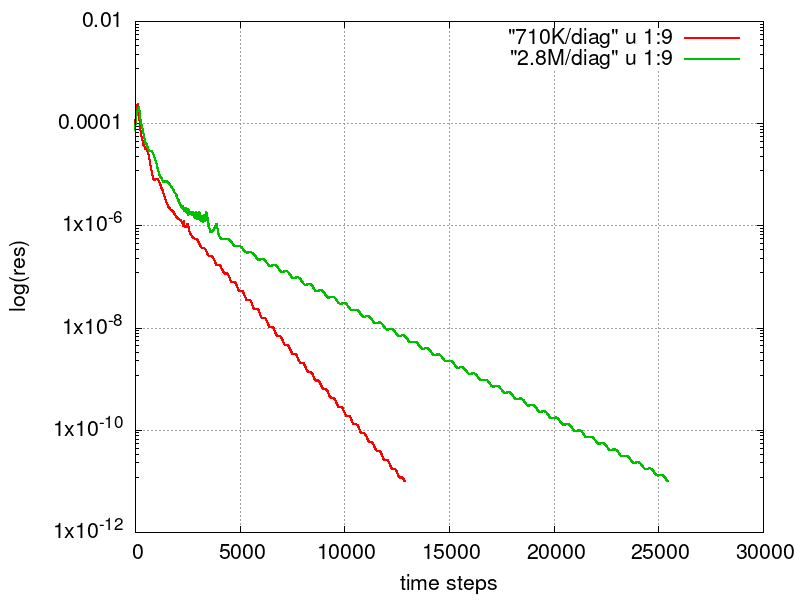
Gnuplot commands to reproduce the above plot:
set terminal png size 800,600 enhanced font "Helvetica,16"
set output "onera_res.png"
set xlabel "time steps"
set ylabel "log(res)"
set logscale y
set grid
plot [] [:1.0e-2] "710K/diag" u 1:9 w l lw 2, "2.8M/diag" u 1:9 w l lw 2
Visualization
ParaView can be used for interactive visualization of the numerically computed 3D fields as
paraview out.e-s.0.30.0Results only on the wing surface can be visualized by first stitching the partitioned surface output files into a single surface output file followed by invoking paraview on the stitched surface exo file:
Main/meshconv -i out-surf.3.e-s.0.30.% -o out-surf.3.exo
paraview out-surf.3.exo
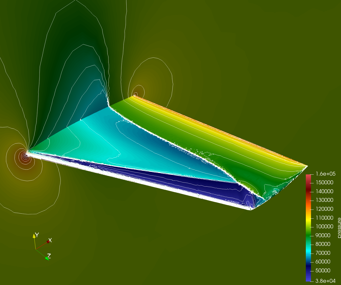
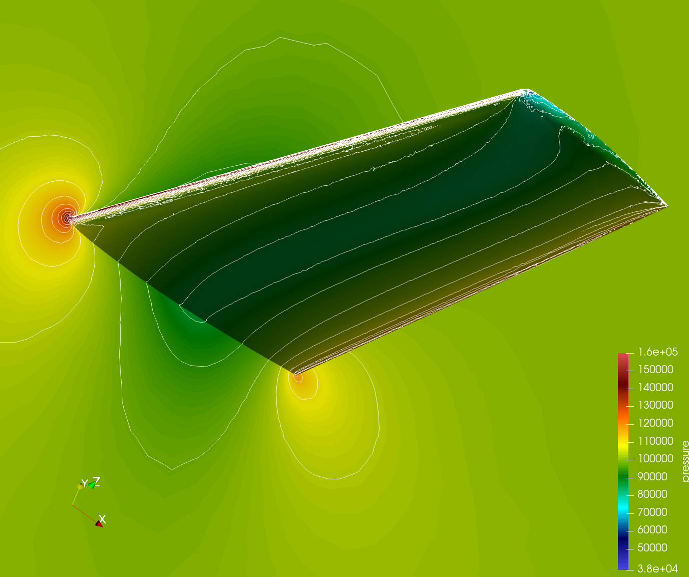
The fine surface mesh is shown in the figure below together with the converged computed pressure contours on the upper and lower surfaces of the wing.
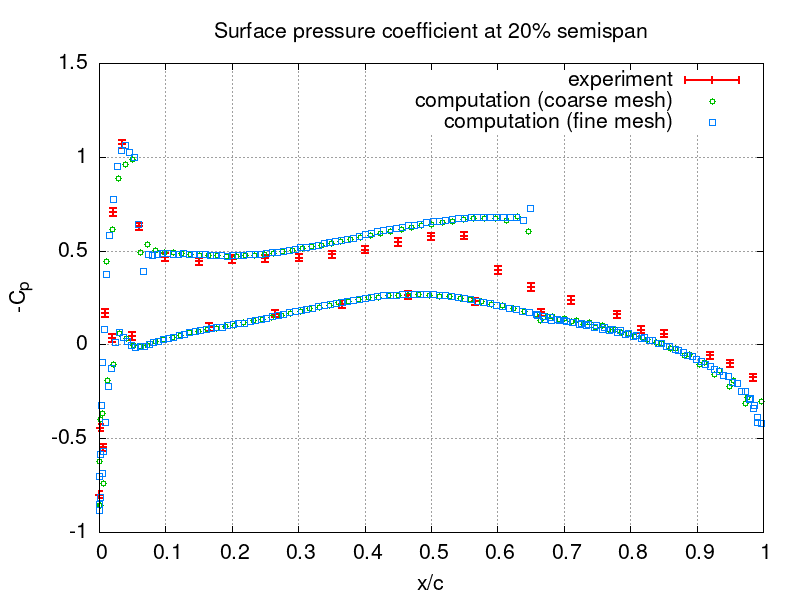
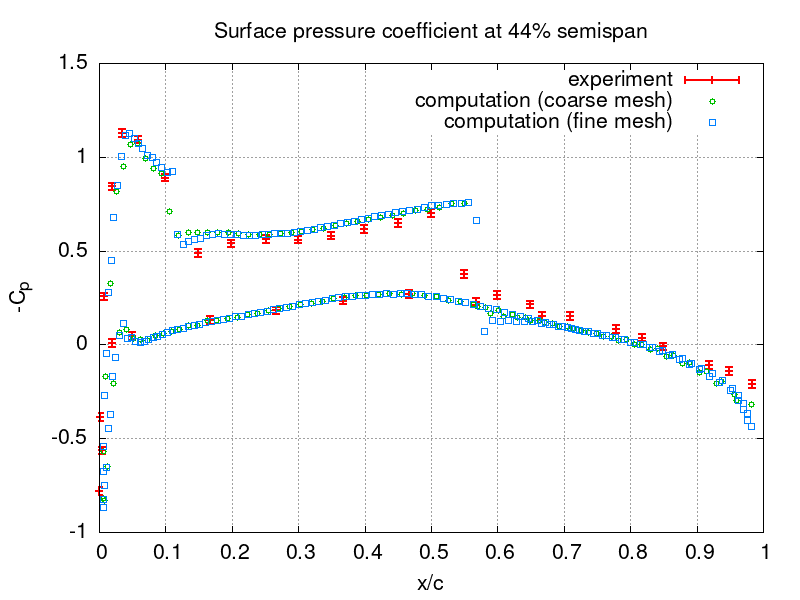
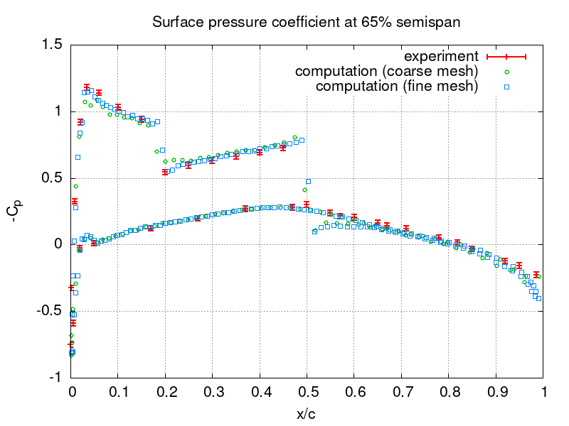
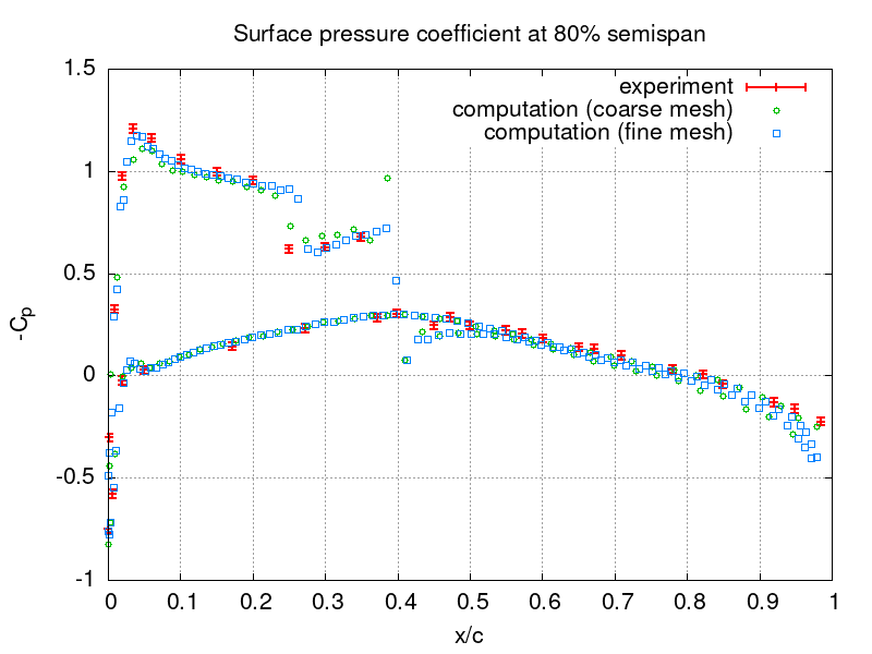
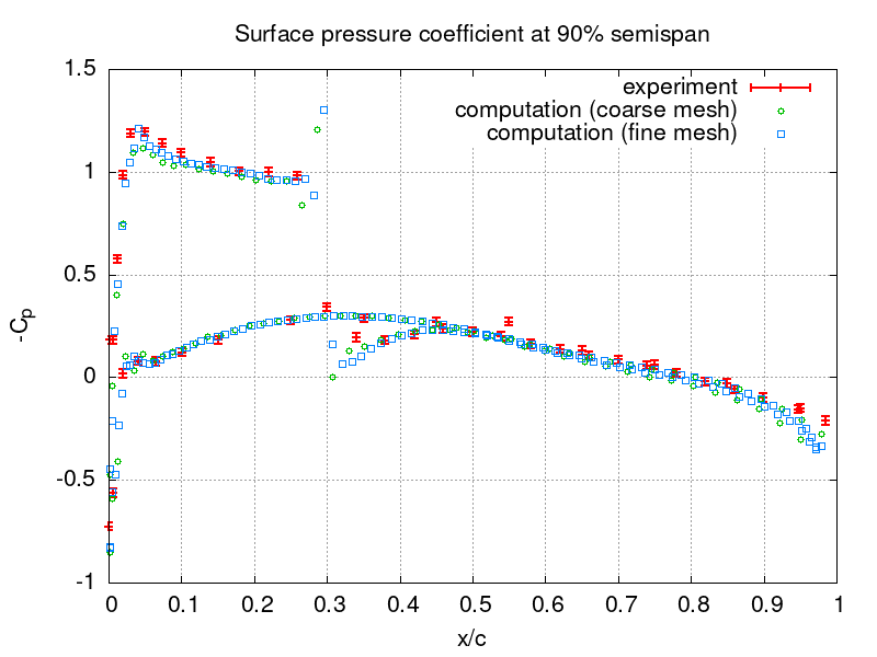
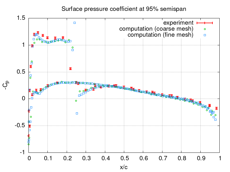
The computed pressure coefficient
distribution is compared to experimental data [3] at various semi-spans in the following figures for both meshes. Here the subscript denotes the far-field conditions, u is the length of the velocity vector, and c is the half-wing span.
Gnuplot commands to reproduce the above plot:
set grid
# coarse and fine mesh, exp with err +/- 0.02
set output "o20.png"; set title "Surface pressure coefficient at 20% semispan"; set xlabel "x/c"; set ylabel "-C_p"; plot [] [:1.5] "expe20.data" u 1:2:(0.02) lw 2.0 w yerrorbars t "experiment", "710K/o20.txt" u (($1-0.115)/0.62):(-($6-1.0e+5)/0.5/1.225/(283.57**2.0+15.159**2.0)) w p pt 6 t "computation (coarse mesh)", "2.8M/o20.txt" u (($1-0.115)/0.62):(-($6-1.0e+5)/0.5/1.225/(283.57**2.0+15.159**2.0)) w p pt 4 t "computation (fine mesh)"
set output "o44.png"; set title "Surface pressure coefficient at 44% semispan"; set xlabel "x/c"; set ylabel "-C_p"; plot [] [:1.5] "expe44.data" u 1:2:(0.02) lw 2.0 w yerrorbars t "experiment", "710K/o44.txt" u (($1-0.25)/0.56):(-($6-1.0e+5)/0.5/1.225/(283.57**2.0+15.159**2.0)) w p pt 6 t "computation (coarse mesh)", "2.8M/o44.txt" u (($1-0.25)/0.56):(-($6-1.0e+5)/0.5/1.225/(283.57**2.0+15.159**2.0)) w p pt 4 t "computation (fine mesh)"
set output "o65.png"; set title "Surface pressure coefficient at 65% semispan"; set xlabel "x/c"; set ylabel "-C_p"; plot [] [:1.5] "expe65.data" u 1:2:(0.02) lw 2.0 w yerrorbars t "experiment", "710K/o65.txt" u (($1-0.373)/0.49):(-($6-1.0e+5)/0.5/1.225/(283.57**2.0+15.159**2.0)) w p pt 6 t "computation (coarse mesh)", "2.8M/o65.txt" u (($1-0.373)/0.49):(-($6-1.0e+5)/0.5/1.225/(283.57**2.0+15.159**2.0)) w p pt 4 t "computation (fine mesh)"
set output "o80.png"; set title "Surface pressure coefficient at 80% semispan"; set xlabel "x/c"; set ylabel "-C_p"; plot [] [:1.5] "expe80.data" u 1:2:(0.02) lw 2.0 w yerrorbars t "experiment", "710K/o80.txt" u (($1-0.46)/0.45):(-($6-1.0e+5)/0.5/1.225/(283.57**2.0+15.159**2.0)) w p pt 6 t "computation (coarse mesh)", "2.8M/o80.txt" u (($1-0.46)/0.45):(-($6-1.0e+5)/0.5/1.225/(283.57**2.0+15.159**2.0)) w p pt 4 t "computation (fine mesh)"
set output "o90.png"; set title "Surface pressure coefficient at 90% semispan"; set xlabel "x/c"; set ylabel "-C_p"; plot [] [:1.5] "expe90.data" u 1:2:(0.02) lw 2.0 w yerrorbars t "experiment", "710K/o90.txt" u (($1-0.517)/0.42):(-($6-1.0e+5)/0.5/1.225/(283.57**2.0+15.159**2.0)) w p pt 6 t "computation (coarse mesh)", "2.8M/o90.txt" u (($1-0.517)/0.42):(-($6-1.0e+5)/0.5/1.225/(283.57**2.0+15.159**2.0)) w p pt 4 t "computation (fine mesh)"
set output "o95.png"; set title "Surface pressure coefficient at 95% semispan"; set xlabel "x/c"; set ylabel "-C_p"; plot [] [:1.5] "expe95.data" u 1:2:(0.02) lw 2.0 w yerrorbars t "experiment", "710K/o95.txt" u (($1-0.546)/0.405):(-($6-1.0e+5)/0.5/1.225/(283.57**2.0+15.159**2.0)) w p pt 6 t "computation (coarse mesh)", "2.8M/o95.txt" u (($1-0.546)/0.405):(-($6-1.0e+5)/0.5/1.225/(283.57**2.0+15.159**2.0)) w p pt 4 t "computation (fine mesh)"
References
- H. Luo, J.D. Baum, R. Lohner, A Fast, Matrix-Free Implicit Method for Compressible Flows on Unstructured Grids, J. Comput. Phys. 146,2, 1998.
- R. Lohner, Applied Computational Fluid Dynamics Techniques: An Introduction Based on Finite Element Methods, Wiley, 2008.
- V. Schmitt, F. Charpin, Pressure Distributions on the ONERA-M6-Wing at Transonic Mach Numbers, Experimental Data Base for Computer Program Assessment, Report of the Fluid Dynamics Panel Working Group 04, AGARD AR-138, 1979.