Examples » ZalCG: Sedov blast

This example uses ZalCG in Inciter to compute the Sedov problem [1], widely used in shock hydrodynamics to test the ability of numerical methods to maintain symmetry. In this problem, a source of energy is defined to produce a shock in a single computational cell at the origin at t=0. The solution is a spherically spreading wave starting from a single point. The semi-analytic solution is known, therefore it can be used to verify the accuracy of the numerical method and the correctness of the software implementation.

Problem setup

We compute the solution in 3D using a simulation domain that is an octant of a sphere, centered around the point {0,0,0}, with increasing mesh resolutions.

The initial conditions are

where and are initial values of the internal energy and pressure respectively, that depend on the size of the control volume at the center of the sphere. As the mesh size is decreased, these values are increased to maintain a constant total energy source. The characteristics of the meshes used are listed in the table below.

Mesh	Points	Tetrahedra	h	e_s	p_s
0	11,304	59,164	0.053	7.25e+3	4.86e+3
1	65,958	362,363	0.029	5.42e+4	3.63e+4
2	505,724	2,898,904	0.014	3.46e+5	2.32e+5
3	3,956,135	23,191,232	0.007	2.78e+6	1.85e+6

Here h is the average edge length. Along the flat faces of the sphere symmetry (free-slip) boundary conditions are applied.

Code revision to reproduce

To reproduce the results below, use code revision 71c6fb2 and the control file below, and adjust for the mesh.

Control file

-- vim: filetype=lua:

print "Sedov blast wave"

term = 1.0
ttyi = 10
cfl = 0.5

solver = "zalcg"
fctsys = { 1, 2, 3, 4, 5 }

part = "rcb"

problem = {
  name = "sedov",
  -- p0 = 4.86e+3        -- sedov_coarse.exo,   V(orig) = 8.50791e-06
  -- p0 = 3.63e+4        -- sedov00.exo,        V(orig) = 1.13809e-06
  -- p0 = 2.32e+5        -- sedov01.exo,        V(orig) = 1.78336e-07
     p0 = 1.85e+6        -- sedov02.exo,        V(orig) = 2.22920e-08
}

mat = { spec_heat_ratio = 5/3 }

bc_sym = {
  sideset = { 1, 2, 3 }
}

diag = {
  iter = 10,
  format = "scientific"
}

fieldout = {
  iter = 1000
}

Run using mesh 3 on 32 CPUs

./charmrun +p32 Main/inciter -i sedov02.exo -c sedov.q -l 1000

Visualization

ParaView can be used for interactive visualization of the numerically computed fields as

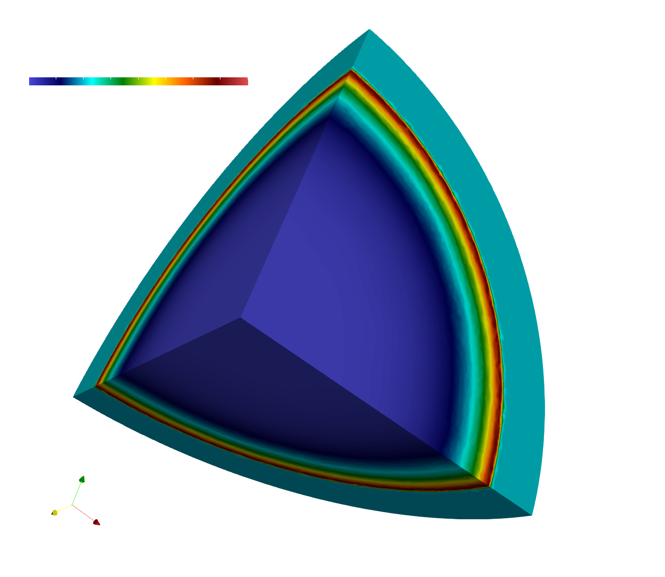
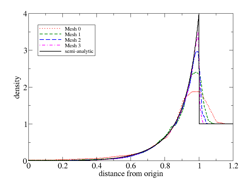
paraview out.e-s.0.32.0

The fluid density on the sphere octant surface using mesh 3 and its radial distributions using different mesh resolutions at t=1.0s are depicted below.

References

[1] L.I. Sedov, Similarity and Dimensional Methods in Mechanics, 10th ed. CRC Press. 1993.