V&V » ZalCG: Urban-scale pollution with deactivation

Deactivation

In some classes of problems the propagating behavior inherent in the equations solved can be exploited to save CPU time by deactivating regions of the computational domain with little to no activity. For example, in supersonic flows the flow field can only be influenced by upstream events. In detonations there is no change in the flow field ahead of the detonation wave. In problems involving scalar transport, e.g., atmospheric pollutant or hazardous material dispersion, a change of the scalar concentration can only occur in donwstream of the source. This last observation is used to invoke a partition-deactivation procedure and demonstrated below to yield considerable savings in CPU time. For an overview of space marching and deactivation methods see [1] and references therein.

Equations solved

In this example we solve the Euler equations coupled to a scalar, representing pollutant concentration, as

where the summation convention on repeated indices has been applied, is the density, is the velocity vector, is the specific total energy, is the specific internal energy, and is the pressure. , , . The system is closed with the ideal gas law equation of state

where is the ratio of specific heats.

Problem setup

We configure the ZalCG solver to compute an urban-scale pollution problem in a typical city whose computational domain contains many of the buildings in downtown Győr, located in North-West of Hungary. The surface mesh is displayed with some of its characteristics in the table below.

Here h is the average edge length.

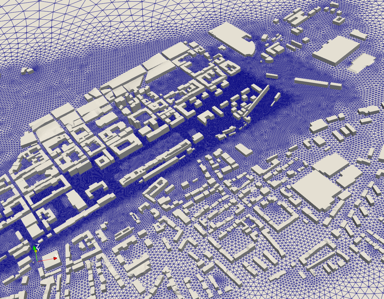Surface mesh for computing an urban-scale pollutatnt dispersion study in the Hungarianc city of Győr.

Initial conditions are specified by atmospheric conditions at sea level at 15C as

and these conditions are also enforced as Dirichlet boundary conditions on the top and sides of the brick-shaped domain during time stepping.

The scalar, , representing pollutant concentration is released from a point source at t=10s of the 140s total time simulated. The value of the scalar is normalized to the constant value of c=1.0 at the source. After verifying that the norms of the velocity component residuals decrease at least two orders in magnitude from their initial values, the flow is assumed to be stationary, the numerical values of density, momentum, and total energy are no longer updated, and the scalar is released.

In the first time step when the scalar is released we deactivate the entire domain. During time stepping partitions gradually reactivate where activity is detected on their boundaries of the active domain. This is combined with overdecomposition, which yields larger number fo partitions compared to the number of CPUs available. Turning on load balancing in Charm++, the dynamically changing heterogeneous parallel load is homogeneized across the simulation. Combining deactivation, overdecomposition, and load balancing yields savings in CPU time.

Code revision to reproduce

To reproduce the results below, use code revision b1a2c26 and the control file below.

Control file

-- vim: filetype=lua:

print "Gyor with scalar"

-- meshes:
-- gyor_m1_10M.exo

scalar_release_time = 10.0

term = 140.0

ttyi = 100
cfl = 0.9

part = "rcb"

solver = "zalcg"
stab2 = true
stab2coef = 0.1

lb = {
  time = scalar_release_time
}

deactivate = {
  sys = { 6 },
  tol = 0.001,
  dif = 0.1,
  freq = 100,
  time = scalar_release_time
}

problem = {
  name = "point_src",
  src = {
    location = { 1914.0, 1338.0, 20.0 },
    radius = 10.0,
    release_time = scalar_release_time,
    freezeflow = 5.0
  }
}

mat = { spec_heat_ratio = 1.4 }

ic = {
  density = 1.225,
  pressure = 1.0e+5,
  velocity = { -10.0, -10.0, 0.0 }
}

bc_dir = {
  { 1, 1, 1, 1, 1, 1, 0 },
  { 9, 1, 1, 1, 1, 1, 0 }
}

bc_sym = {
  sideset = { 10, 21, 22, 23, 24 }
}

fieldout = {
  iter = 10000,
  time = 10.0,
  sideset = { 10, 21, 22, 23, 24 },
  --range = {
  --  { scalar_release_time, term, 10.0 }
  --}
}

diag = {
  iter = 100
}

Run on multiple compute nodes

# no deactivation, no overdecomposition, no load balancing
./charmrun +p $((32*$SLURM_NNODES)) Main/inciter -c gyor3dea.q -i gyor_m1_10M.exo
# deactivation + overdecomposition (u=0.55) + load balancing (invoke the 'MetisLB' in the first LB step then the 'GreedyRefine' strategy in every 100th time step)
./charmrun +p $((32*$SLURM_NNODES)) Main/inciter -c gyor3dea.q -i gyor_m1_10M.exo -u 0.55 -l 100 +balancer MetisLB +balancer GreedyRefineLB

Numerical results

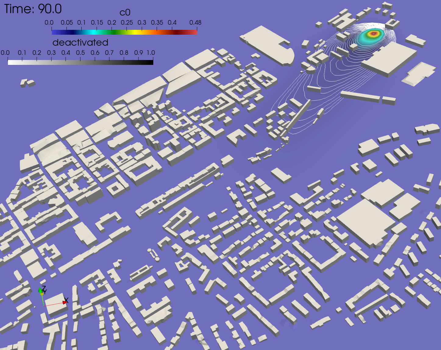
The figures below depicts the ground-level concentrations at t=90s to allow comparing simulations without overdecomposition, deactivation or load balancing (on 128 mesh partitions) and with overdecomposition, deactivation and load balancing (on 284 mesh partitions). The numerical solutions are nearly indistinguishable.

Surface distributions of a propagating scalar representing pollutant concentration in an urban-scale air quality study with stationary winds, computed on 4 networked compute nodes on 128 CPUs without deactivation, overdecomposition or load balancing using 128 mesh partitions.

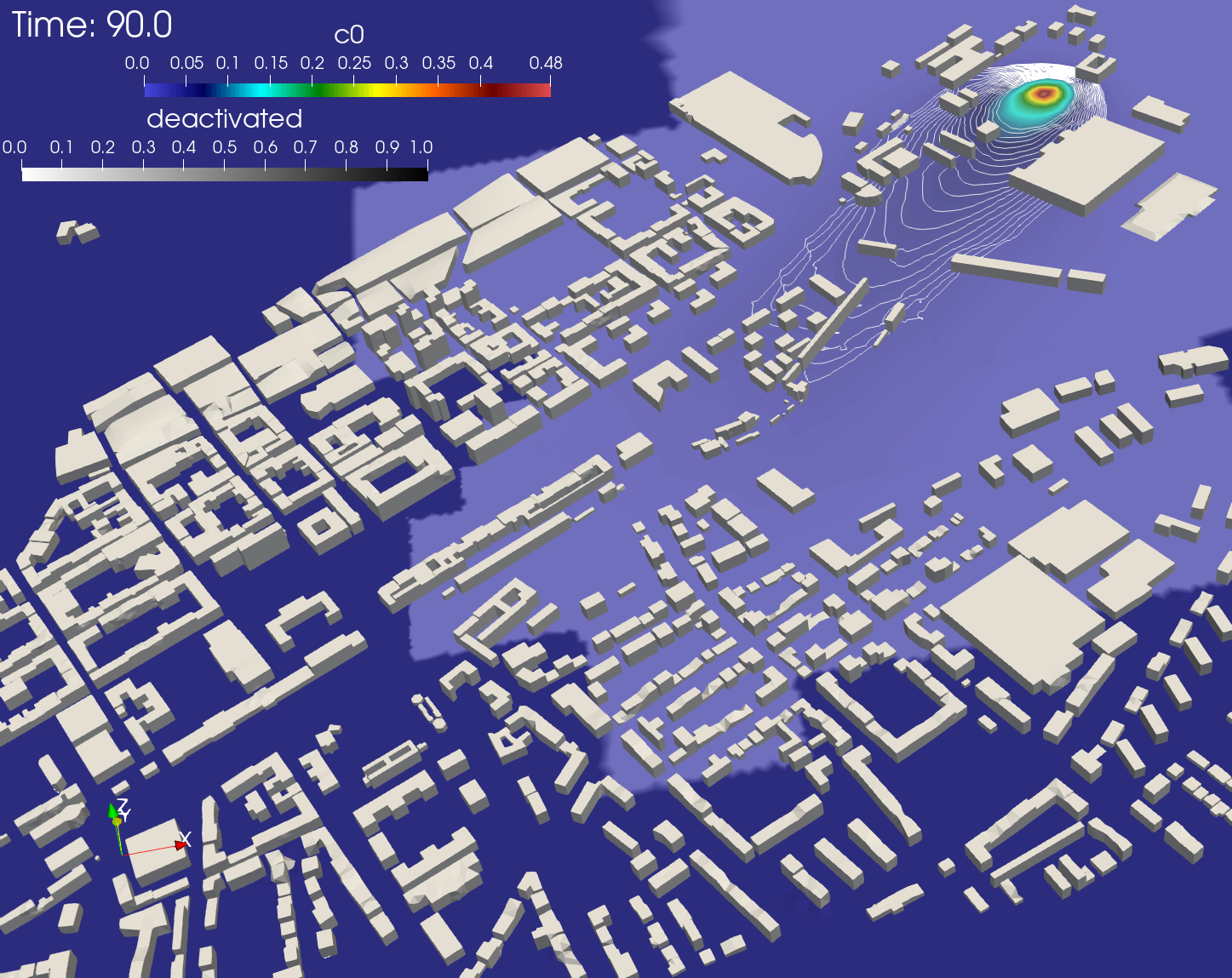Surface distributions of a propagating scalar representing pollutant concentration in an urban-scale air quality study with stationary winds, computed on 4 networked compute nodes on 128 CPUs with deactivation, overdecomposition and load balancing yielding 284 mesh partitions. Superimposed in bright blue color is the deactivation state of the partitions.

Computational cost

The figres below show the time evolution of the computational cost of a single time step during the urban-air pollution calculations, comparing the baseline with 128 partitions without deactivation, overdecomposition or load balancing to that of deactivation, overdecomposition, and load balancing with 284 partitions. The wall-clock time of a time step is measured on the vertical axis in milliseconds, while the elapsed wall-clock time is on the horizontal axis. The runs with deactivation, overdecomposition, and load balancing outperform the baseline case (without deactivation, overdecomposition or load balancing). This is indicated by the green-dashed line finishing earlier and staying below the red-dotted line. Though both simulations advance until the same physical time of t=140s, the elapsed wall-clock time is approximately half with deactivation.

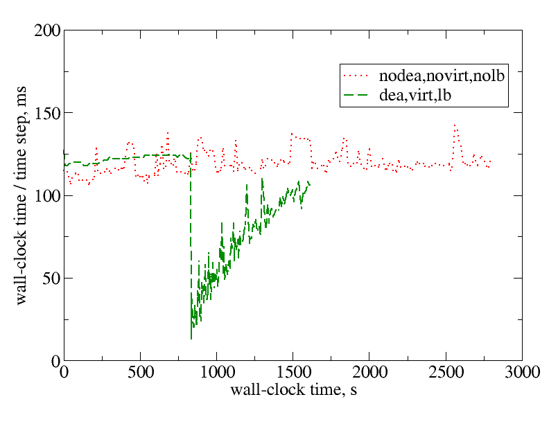Wall-clock times for each time step measured in milliseconds during computation of the urban-air pollution problem without deactivation, overdecomposition or load balancing and with deactivation, overdecomposition, and load balancing until the same physics time t=140s.

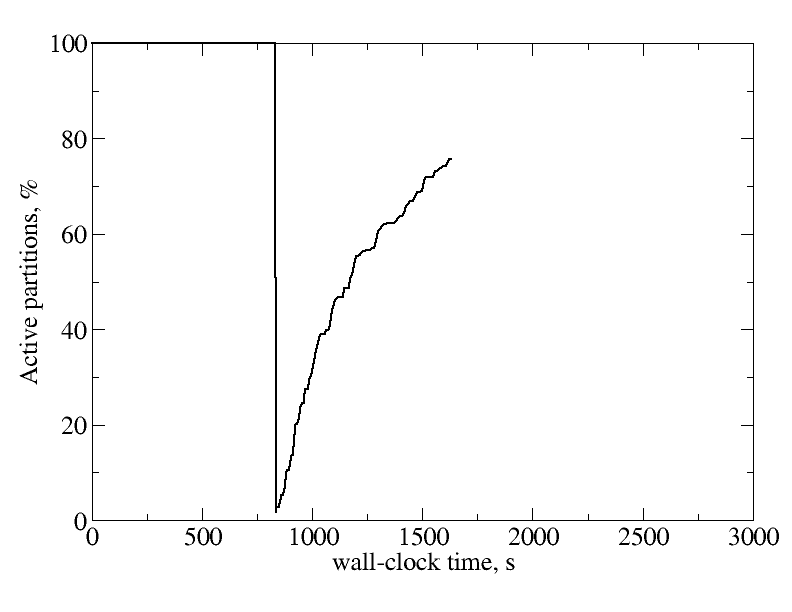Fraction of active partitions in wall-clock time computing the urban-scale pollution problem with deactivation, where 100% indicates the initial stage of converging the flow field to a steady state, after which the scalar is released into a flow in which the hydrodynamics variables are no longer updated.

Another way to measure the effectiveness of the deactivation procedure is to plot wall-clock times with deactivation, overdecomposition, and load balancing relative to wall-clock times without deactivation, overdecomposition, or load balancing as a function of the physics time integrated. This is plotted below.

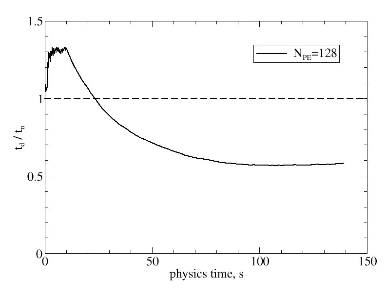
When this ratio is below 1.0, the deactivation procedure outperforms the original calculations, as measured by wall-clock times. The figure shows that until the scalar is released, , the simulation with deactivation is approximately 30% slower than that with no deactivation. This is not due to the cost of the deactivation procedure or load balancing, since these parts of the algorithm are not yet invoked. The increased cost is due to the increased communication cost due to overdecomposition, i.e., using 284 mesh partitions instead of 128. After the scalar is released, almost the entire domain is deactivated and the simulation speeds up significantly. As the figure shows, even though more and more partitions become active, the ratio of wall-clock times stays below unity, attesting to the effectiveness of the procedure.

References

1. R. Lohner, Applied Computational Fluid Dynamics Techniques: An Introduction Based on Finite Element Methods, Wiley, 2008.