V&V » ZalCG: Sedov blast with deactivation

Deactivation

In some classes of problems the propagating behavior inherent in the equations solved can be exploited to save CPU time by deactivating regions of the computational domain with little to no activity. For example, in supersonic flows the flow field can only be influenced by upstream events. In problems involving scalar transport, e.g., atmospheric pollutant or hazardous material dispersion, a change of the scalar concentration can only occur in donwstream of the source. In detonations there is no change in the flow field ahead of the detonation wave. This last observation is used to invoke a partition-deactivation procedure and demonstrated below to yield considerable savings in CPU time. For an overview of space marching and deactivation methods see [1] and references therein.

The Sedov problem with deactivation

We configure the ZalCG solver in Inciter to compute the Sedov problem [2] using deactivation. In this problem, a source of energy is defined to produce a shock in a single computational cell at the origin at t=0. The solution is a spherically spreading wave starting from a single point. We used a domain that is eighth of a sphere with the mesh consisting of 23,191,232 tetrahedra and 3,956,135 points. See also ZalCG: Sedov blast for more details on the problem setup.

After domain decomposition before time stepping starts we deactivate the entire domain during setup. During time stepping partitions gradually reactivate where activity is detected on their boundaries of the active domain. This is combined with overdecomposition, which yields larger number fo partitions compared to the number of CPUs available. Turning on load balancing in Charm++, the dynamically changing heterogeneous parallel load is homogeneized across the simulation. Combining deactivation, overdecomposition, and load balancing yields savings in CPU time.

Code revision to reproduce

To reproduce the results below, use code revision 5892d62 and the control file below.

Control file

-- vim: filetype=lua:

print "Sedov blast wave with deactivation"

term = 1.0
ttyi = 10
cfl = 0.5

solver = "zalcg"
stab2 = true
stab2coef = 0.1
fctsys = { 1, 2, 3, 4, 5 }

deactivate = {
  sys = { 1 },
  tol = 0.005,
  dif = 0.5,
  freq = 5
}

part = "rcb"

problem = {
  name = "sedov",
    p0 = 1.85e+6
}

mat = { spec_heat_ratio = 5/3 }

bc_sym = {
  sideset = { 1, 2, 3 }
}

diag = {
  iter = 1,
  format = "scientific"
}

fieldout = {
  iter = 100
}

Run on multiple compute nodes

# no deactivation, no overdecomposition, no load balancing
./charmrun +p $((32*$SLURM_NNODES)) Main/inciter -c sedov.q -i sedov02.exo
# deactivation + overdecomposition (u=0.5) + load balancing (invoke the 'GreedyRefine' strategy in every 100th time step)
./charmrun +p $((32*$SLURM_NNODES)) Main/inciter -c sedov.q -i sedov02.exo -u 0.5 -l 100 +balancer GreedyRefineLB

Numerical results

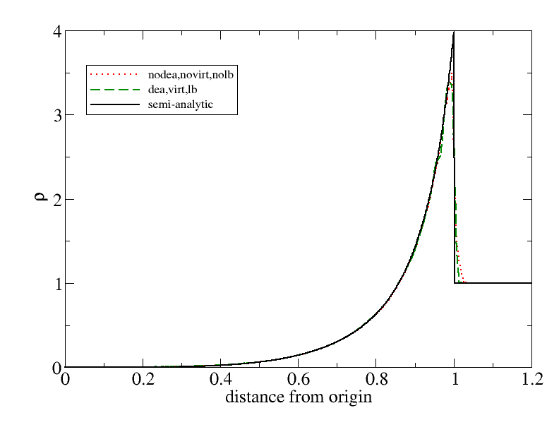
The figure below shows the computed density field at t=1.0 extracted from the 3D field along a radial line starting from the origin with and without deactivation. The results are nearly indistinguishable.

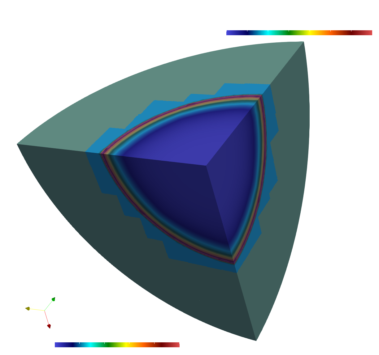
The next figure shows the surface density with the superimposed deactivation status during simulation. Inactive regions ahead of the wave are in dark green, active regions are bright green.

CPU timings

The following figures depict the evolution of the computational cost during time stepping on 6 compute nodes (each with 32 CPU cores), comparing the runs with and without decativation, computing the same problem configured the same way using the same mesh until the same physics time t=1.0. As the figures show, the simulation with deactivation takes about half the time compared to the one without deactivation if one integrates time until t=1.0. However, the relative computational cost in general will depend on how far in time the wave needs to be propagated.

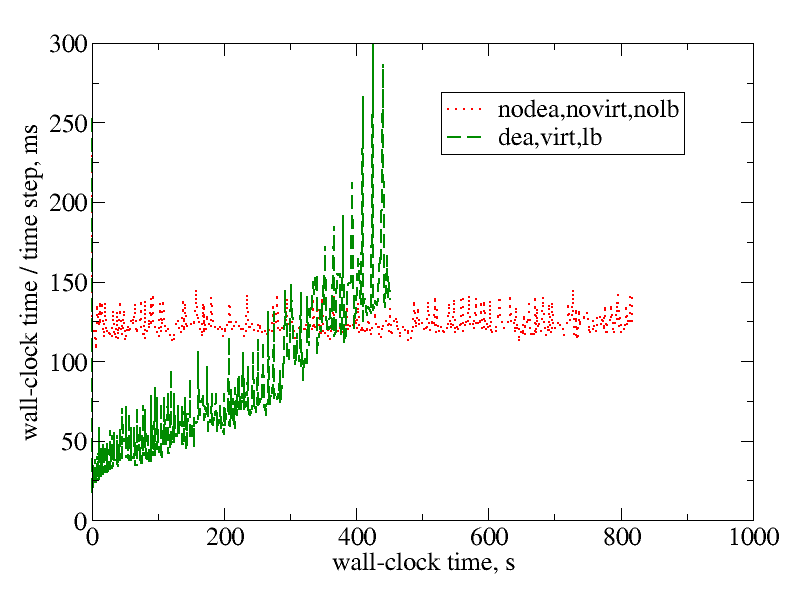Wall-clock times for each time step in milliseconds during computing the Sedov problem until (physics time) t=1.0 with and without deactivation.

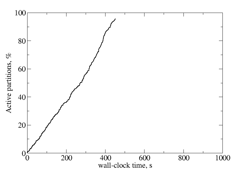Fraction of active partitions in wall-clock time computing the Sedov problem with deactivation.

Another way to measure the effectiveness of the deactivation procedure is to plot wall-clock times with deactivation, overdecomposition, and load balancing relative to wall-clock times without deactivation, overdecomposition, or load balancing as a function of the physics time integrated. This is plotted below.

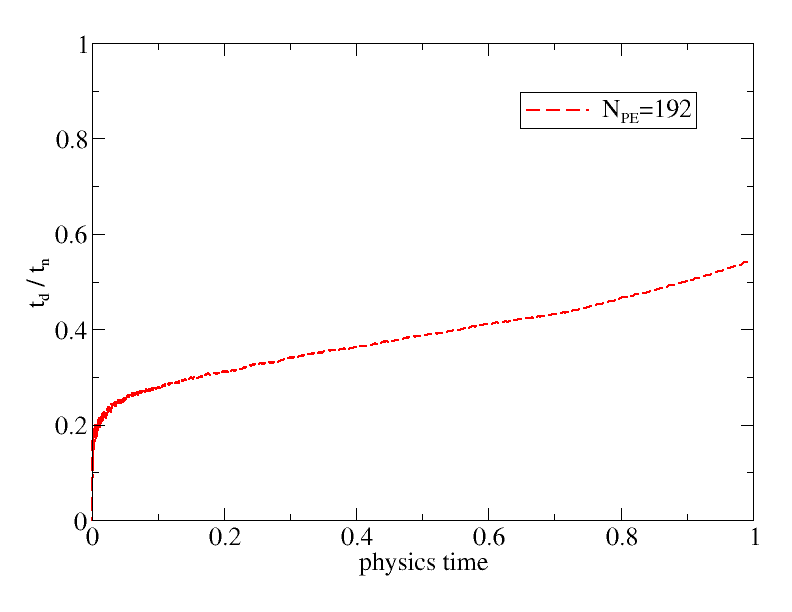
As long as this ratio stays below 1.0, the deactivation procedure outperforms the original calculations, as measured by wall-clock times. The figure shows that the simulation with deactivation consistently outperforms its counterpart without deactivation during the entire physics time, , integrated.

References

1. R. Lohner, Applied Computational Fluid Dynamics Techniques: An Introduction Based on Finite Element Methods, Wiley, 2008.
2. L.I. Sedov, Similarity and Dimensional Methods in Mechanics, 10th ed. CRC Press. 1993.